Where the series stands
My drawing arm needs to learn as it changes. It also needs to react to errors that change within a stroke. Those are different jobs. A correction learned from past drawings handles the repeatable part. Feedback handles what the arm does differently this time.
This is part 7 of the SO-101 series. Part 6 measured the pen tip with a tablet. A frozen learned correction reached 1.057 mm RMS on the controller-selection drawings (Measured). RMS means square each distance error, average, then take the square root. A large miss counts more than a small one.
Since then, I tried direct motor drive, added learning, and tested the software copy of the arm against more recordings. I made an explainer for a friend who works on robots. This post follows that explainer, with the later results and corrected numbers.
The main result is a clearer error budget. The encoders explain about 70% of the variation between repeated runs in the studied cohort (Offline). That gives feedback a useful signal. The learning tests also show why I must score timing and drawing error separately.
What the one-millimeter numbers mean
I need to separate error against the target from variation between runs. An arm can draw the same wrong line every time. It can also draw a different line each time, with an average close to the target.
| Quantity | Result | What it measures |
|---|---|---|
| Pen minus target, part 6 frozen correction | 1.057 mm RMS, Measured | How far the selected controller's drawings were from the requested path |
| One repeat minus another | 0.95 mm RMS, Offline | Difference between recorded runs of the same motion with the same settings, pooled over 96 pairs |
| Inferred variation of one run | About 0.67 mm RMS, Offline | The pairwise spread divided by the square root of two |
| One run minus the repeat mean, separate cohort | 0.72 mm RMS, Offline | Variation around the mean of 50 runs of the same practice scribble |
The board calls the pairwise result a repeat floor. It describes variation in those recordings. It does not say that the arm controls its pen to within a millimeter.
The per-run estimate and the separate repeat-mean result put variation at about 0.67 to 0.72 mm RMS (Offline) in those cohorts. This range combines different analyses. It is not a confidence interval.
A fixed correction can remove a repeatable bias. It cannot know which way the next run will deviate. That is why the distinction changes the next experiment: teach the average error between runs, and use feedback to respond during the run.
Direct drive: taking over the motor command
The controllers in the earlier parts send position goals to the servos. Each servo then runs its own position loop. My controller works around that loop's friction, delay and internal motion rules.
Direct drive changes this boundary. I send a motor duty command to the pan, the joint that turns the whole arm about its base. Duty is the fraction of time the motor drive applies power. My loop reads the encoder and chooses that command. This gives me control over a part of the system that a position goal leaves inside the servo.
The pan reached 1.68 mrad RMS tracking error at a 12% duty limit on 13 Oct (Measured). That is an angle error for one joint. It is not the tablet's pen error. The corrected score compares the encoder with the reference at the time of the reading. The explainer's earlier value used the reference at the command's aim time.
More steady duty did not help in that test. At a 20% limit, pan tracking error was 3.91 mrad RMS (Measured). The joint entered a limit cycle: the correction kept driving it back and forth.
The arm then changed. On 14 Oct, runs at the 12% limit gave 3.08 and 10.40 mrad RMS (Measured) as the pan needed more drive to break free. This makes the next design question concrete: apply enough drive to start motion, then reduce it before the joint overshoots.
Direct drive remains a candidate. Its place on the ladder depends on a completed tablet comparison against the current controller.
Learning between drawings
The correction in part 6 was frozen. I fit it from tablet recordings, then left its weights fixed while the arm drew. A small neural network added another correction on top. In the early comparisons, that frozen network reduced nib RMS by 0.23 and 0.20 mm against the part 6 correction (Measured) on the controller-selection drawings.
That result made the next step clear: update the correction as more practice data arrives. The loop is simple.
- Draw a practice scribble and record the requested path, joint angles and tablet path.
- Fit the correction on practice data.
- Freeze it and score the Test drawings: kitten, star, spiral and square.
- Use separate validation drawings to report generalization.
The Test drawings choose controllers. They do not train the correction. Validation drawings do neither.
Online learning means that the deployed learner keeps updating from new practice. Its useful score is the error it maintains over time, as friction, temperature and the nib change. A low point early in a run does not establish that long-run performance.
Timing and drawing error need separate scores
The later frozen-head test exposed a scoring trap. A correction can make the pen arrive sooner and still draw a worse path after I account for that timing change.
The example below uses a head trained on 64 practice motions, with 102 training passes, then evaluated on the real arm. Each Test drawing ran in a physics baseline, head, physics baseline order. I compare the head with the mean of the baselines on either side.
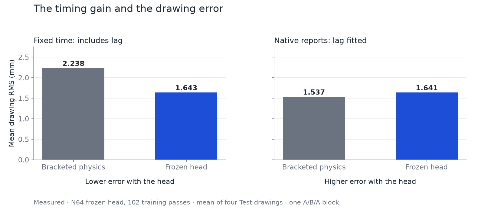
At fixed time, the head reduced RMS from 2.238 to 1.643 mm (Measured). That score asks where the pen was when it should have been at each target point.
Using the tablet's native report times and fitting the lag, RMS went from 1.537 to 1.641 mm (Measured). That score removes a constant timing offset, retains spatial bias, and uses no rigid spatial fit. On this measure, the head was worse.
So the timing gain is real in that block. A drawing-quality gain after fitting the lag was not shown. I now report both scores. I also keep this frozen-head experiment separate from the online-learning curve that the project still needs to complete.
Feedback during a stroke
Learning the mean leaves a second question: which part of a run's deviation can the encoders tell me about now?
An Offline analysis took 40 repeats of one practice scribble, with the old nib, the physics controller and fixed servo gains. It subtracted the mean path from each run. The tablet's remaining deviation was 0.69 mm RMS (Offline).
Joint-angle signals explained about 70% of that variance, leaving about 30% unexplained (Offline). These are shares of squared deviation. They are not distances that I can add. The wrist-flex joint made the largest contribution in this cohort.
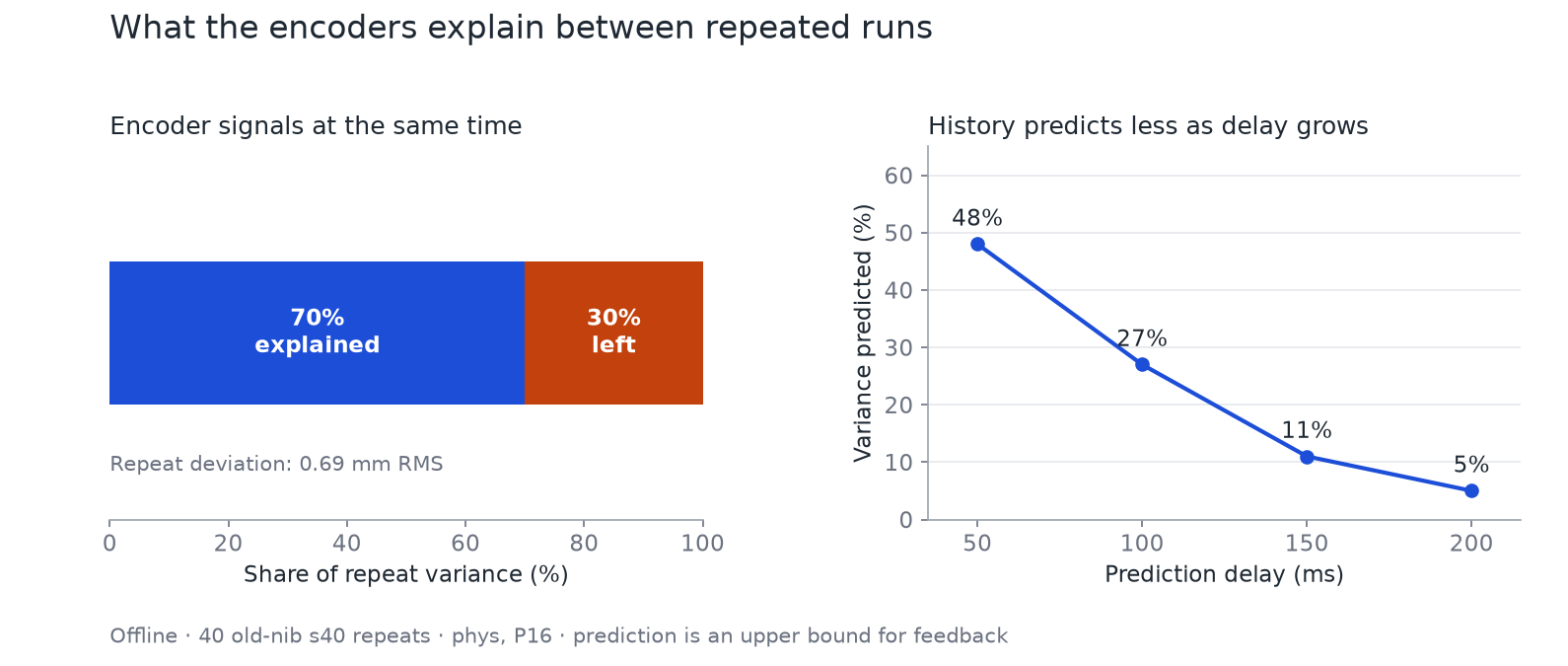
This corrects an early statement in the explainer. The encoders do not miss most of the run-to-run variation in this study. They see much of it.
Delay determines how much of that signal a controller can use. With a 100 ms prediction delay, encoder history explained 27% of the variance, corresponding to a reduction from 0.71 to 0.61 mm RMS in the stroke-only analysis (Offline). That is a prediction bound from recordings. The next arm test must establish what a closed loop can remove.
The two forms of learning now have distinct roles. Between drawings, update the correction for the repeatable error and slow changes. During a stroke, use recent joint readings to respond to the current deviation. The latter must use only readings that have already arrived.
The twin must match the error at the right time
The twin is a software copy of the arm. It runs the controller against a model of the joints and a virtual tablet. It includes pen contact, friction and compliance, which lets the pen trail as it bends under drag. A learned residual can add the part that the physics model misses.
A useful twin must reproduce where the real arm misses. Drawing a line with the right overall RMS is insufficient: the twin could miss on the opposite side of the target.
I score the share of the arm's squared pen error that the twin reproduces, sample by sample. A perfect match gets all of it. Predicting zero arm error gives zero share. A negative share means the twin's prediction is worse than that zero-error prediction.
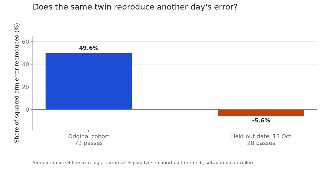
Adding a fitted term with the shape of mechanical play brought the twin to 49.6% share on the original cohort (Simulation compared with Offline logs). The same version gave −5.6% on the held-out date. Its RMS mismatch with the arm was 1.30 and 1.25 mm, respectively, under that study's alignment convention. The share fell even though the absolute mismatch was similar, because the arm's error was smaller in the later cohort.
This is a transfer test the twin failed. The fitted play term improves the model, but it does not identify a physical gear gap by itself. The next model work must separate geometry, contact and breakaway friction, then test on data that the fit did not use.
What hardware comes next
The error budget gives each proposed part a job.
- Motion sensors on the arm. The IMU set is ordered. An accelerometer can test the shaking and bending that the rigid joint model misses. It needs comparison with the tablet before it becomes a controller input.
- A spring scale and pen tests. The planned measurements are lateral pen stiffness and drag. They give the contact model physical inputs instead of values chosen only to fit a path.
- Pan settings and mechanics. The direct-drive results call for a breakaway test and a fair drawing comparison. Extra steady power already produced oscillation in one test. Changing the drive around breakaway and changing the mechanical friction are separate candidates.
- A calibration station. Outside cameras and known touch points on the table could check geometry and tool position. This remains an idea for periodic calibration. A station would not measure every error during a stroke.
For the controller, I favor the combination of a learned mean correction and causal encoder feedback. Updating only between drawings leaves the current deviation. Direct drive gives more control over the servo behavior, but still needs a completed pen-error comparison. The weakest point of the combined approach is delay: a useful signal can arrive too late for a correction to help.
Limits
- The repeat studies use specific drawings, poses, gains and nibs. Their spread is not a universal hardware floor. The inferred per-run value assumes independent deviations with comparable variance.
- The encoder-visible share concerns variation around a repeat mean in the old-nib cohort. It does not partition all target error. The prediction bound excludes interactions with the existing control loop.
- The later frozen-head comparison has one bracketed block per head. Baseline drift and unequal training passes prevent a causal scaling conclusion. The matched-count online deployment experiment is incomplete.
- Direct drive has no completed tablet result that establishes a win over the current controller. Joint-angle tracking alone cannot rank pen precision.
- The twin's date test changes several conditions together. Its share also depends on the size of the real arm's error. Simulation results do not rank real controllers.
- General motion in three dimensions, changing payloads, a working IMU correction and a calibrated station remain untested here.
Where the numbers come from
Measured means the real arm ran. Offline means analysis of recorded arm data. Simulation means the software arm. A Dry run checks software paths without establishing arm precision. Only Measured comparisons rank controllers.
The claim check records the source file, version, metric and cohort for each precision number. The figure data contains the frozen summary values used in the plots.
Check yourself
Question 1. An Offline analysis finds that two runs differ by 0.95 mm RMS. Does that prove either one stayed within 0.95 mm of the target?
Answer
No. Both runs can share a large error against the target. Their difference measures variation between them. The target error needs a separate comparison with the requested path.
Question 2. A learned correction lowers the fixed-time error, but raises the error after fitting the lag. What did the test show?
Answer
It showed a gain in the score that includes timing. It did not show better drawing accuracy after fitting the lag. Keep both scores and test the next correction against both.