Six ways to choose the goal

Part 1 ended with one equation for a joint of my arm, and one rule: the servo only makes torque from the gap between the goal and the joint, so every term of the equation needs a bit more gap. Part 2 was about the reading the controller sees. This part is about the fixes.

I built close to twenty controllers during this project, and each one has a short lab name. Taken one by one, they look like a long list of small variations. They become much simpler once you write them all as one formula for the goal: each controller is that formula with some terms switched on and the others set to zero. They fall into six families, and each family exists to solve one kind of problem from the equation of part 1.

One formula for the goal

Part 1 gave the ideal goal, if I knew every term of the joint equation exactly:

\text{goal}(t) = q^*(t + D) + \frac{M\ddot q^* + G + d\,\dot q^* + f\,\text{sign}(\dot q^*) + C\,\dot q^*}{k_p}

I don't know the terms exactly, so a real controller uses estimates, written with a hat ( $\hat M$ , $\hat G$ and so on). It can also correct the goal from the error it measures, and from what it learned on earlier runs. With all of that, one formula covers every controller in this series:

\text{goal}(t) = q^*(t + T) + \frac{\hat M\ddot q^* + \hat C\dot q^* + \hat G(q^*) + \hat d\,\dot q^* + \hat f\,\text{sign}(\dot q^*)}{k_p} + \hat w + K_P\,e + K_I\!\int e\,dt + u_k

Each new term has one meaning:

$T$ is the look-ahead: how far ahead on the target path the controller reads. $T = D$ cancels the dead time.
$\hat w$ is a disturbance estimate: a running guess of the torque the model is missing, already divided by $k_p$ so it is in goal units. A payload is the typical example.
$e = q^* - \hat q$ is the error the controller measures. $K_P$ and $K_I$ are the gains of the proportional and the integral feedback.
$u_k$ is a correction learned for step $k$ of a motion, from earlier runs of the same motion.

The widget shows the formula. Select a family, then a controller: the terms that the controller uses stay bright, and the others are set to zero.

goal(t) = q*(t + T) + (M̂ q̈* + Ĉ q̇* + Ĝ(q*) + d̂ q̇* + f̂ sign(q̇*)) / kp + ŵ + K_P e + K_I ∫e dt + u_k. direct: every term is 0. lead: T = one step. inv: T = 33 ms, d̂/kp = 0.106 s, M̂/kp = 0.0023 s². sag and grav: inv + Ĝ. pi: inv + K_P = 0.2, K_I = 2 per second. adapt: inv + ŵ from a Kalman filter. solve, mpc, mpca: a servo model with T, M̂, d̂, Ĝ, the dead band and ŵ, inverted by search. ilc: inv + u_k. The network: T = one step, the τ̂/kp part learned from data, K_P = -0.25, K_I = 3.

The table gives the same information for every controller. Part 1 defines the terms.

Controller	Family	$T$	$\hat\tau/k_p$ terms	$\hat w$	$K_P$ , $K_I$	$u_k$	Goal found by
`direct`	1	0	none	0	0, 0	0	formula
`lead`	2	1 step	none	0	0, 0	0	formula
`inv`	2	$D$	$\hat d$ , $\hat M$ , fitted on a step test	0	0, 0	0	formula
`sag`	3	$D$	as `inv`, plus $\hat G$ fitted on holds	0	0, 0	0	formula
`grav`	3	$D$	as `inv`, plus $\hat G$ from MuJoCo	0	0, 0	0	formula
Classical	3	1 step	$\hat M$ , $\hat G$ , $\hat d$ , $\hat f$	0	4, 10	0	formula
`pi`	4	$D$	as `inv`	0	0.2, 2	0	formula
`pisag`	4	$D$	as `sag`	0	0.2, 2	0	formula
`adapt`	4	$D$	as `inv`	Kalman filter	0, 0	0	formula
`rls`	4	$D$	re-fitted during the run	0	0, 0	0	model inverse
`solve`	5	in the model	servo model: $\hat M$ , $\hat d$ , $\hat G$ , dead band	slow estimate	0, 0	0	search, 0.25 s ahead
`mpc`	5	in the model	as `solve`	slow estimate	0, 0	0	search, 0.25 s plan
`mpca`	5	in the model	as `solve`	Kalman filter	0, 0	0	search, 0.25 s plan
Fitted	5	1 step	all, from a fitted MuJoCo copy	0	0, 3	0	Newton, one step
`ilc`	6	$D$	as `inv`	0	0, 0	learned	formula
`ilcmpc`	6	in the model	as `solve`	slow estimate	0, 0	learned	search, 0.25 s plan
Network	6	1 step	learned by a network	0	−0.25, 3	0	formula

Two things in this table aren't a plain "switch a term on". First, the integral $K_I\!\int e\,dt$ and the estimate $\hat w$ do the same job: both build up, during the run, the steady goal offset that the model misses. The integral is the simplest possible estimator of a constant $\hat w$ . A Kalman filter is a better one, because it uses a model to tell a load from a sag from noise. Second, the planners in family 5 use the same terms, but they don't add them up. The servo has parts with no formula inverse: the dead band, the ticks, the goal hold and the torque limit. So the planners simulate a model of the servo for many candidate goals and keep the best one.

Six families, six problems

This table gives each family, the problem it solves, and the controllers in it. The families differ only in the problem they attack.

Family	Problem it solves	Controllers
1. Do nothing	Nothing. It is the baseline that shows every problem.	`direct`
2. Look ahead in time	The goal acts late: dead time, goal hold, and the lag from wet friction.	`lead`, `inv`
3. Add the forces you know	Forces you can compute before the run: gravity, inertia, friction.	`sag`, `grav`, Classical, preview
4. Estimate what you don't know	Forces you can't compute before the run: a payload, wear, model error.	`pi`, `pisag`, `adapt`, `rls`
5. Plan with a servo model	Parts with no formula inverse: the dead band, ticks, the goal hold and the torque limit.	`solve`, `mpc`, `mpca`, Fitted
6. Learn from repeats or data	Errors that repeat on the same path, or that the form of the model misses.	`ilc`, `ilcmpc`, the network

Many controllers combine two families. pi is the inv look-ahead plus feedback, and mpca is a planner plus a Kalman estimate. I put each controller in the family of the part it adds.

I tested these controllers in two places. On my real arm, I ran them on recorded motions such as "cat", a test motion of 120 s. In a simulation study, I ran five ways of choosing the goal on 96 test paths of 6 s each, against a simulated robot whose true numbers I know.

Real arm on the cat motion with one controller from each of three families: `direct` (family 1) at 30 Hz, `pi` (family 4), `solve` and `mpc` (family 5) at 60 Hz, so the loop rate is part of the difference. The error is drawn 10 times larger, and large errors are compressed so the arm stays clear of the table and the base. The gray shape is the target pose. The red line joins the gripper tip to where the tip should be. The plot under each arm gives the true joint error in mrad, with the same scale in every plot. The numbers cover this 16 s window only. Open video

Bar chart of the real-arm tracking error. Cat motion: direct 22.5 mrad at 30 Hz, pi 8.4, solve 6.2 and mpc 6.0 at 60 Hz. Signature motion: direct 28.3, lead 23.7 and inv 13.4 mrad. — Real arm, RMS error over all five joints and the whole motion. The two motions are different, so compare bars within a motion.

Simulation, log scale: out of the box 37.2 mrad, Classical model plus PID 1.117, neural network 0.446, Fitted servo model 0.398 and Exact model 0.398. A dashed line marks the one-reading rounding RMS of 0.443 mrad. — Simulation, fixed test set of 96 paths that no controller saw during tuning. The best controllers land below the RMS of one rounded reading.

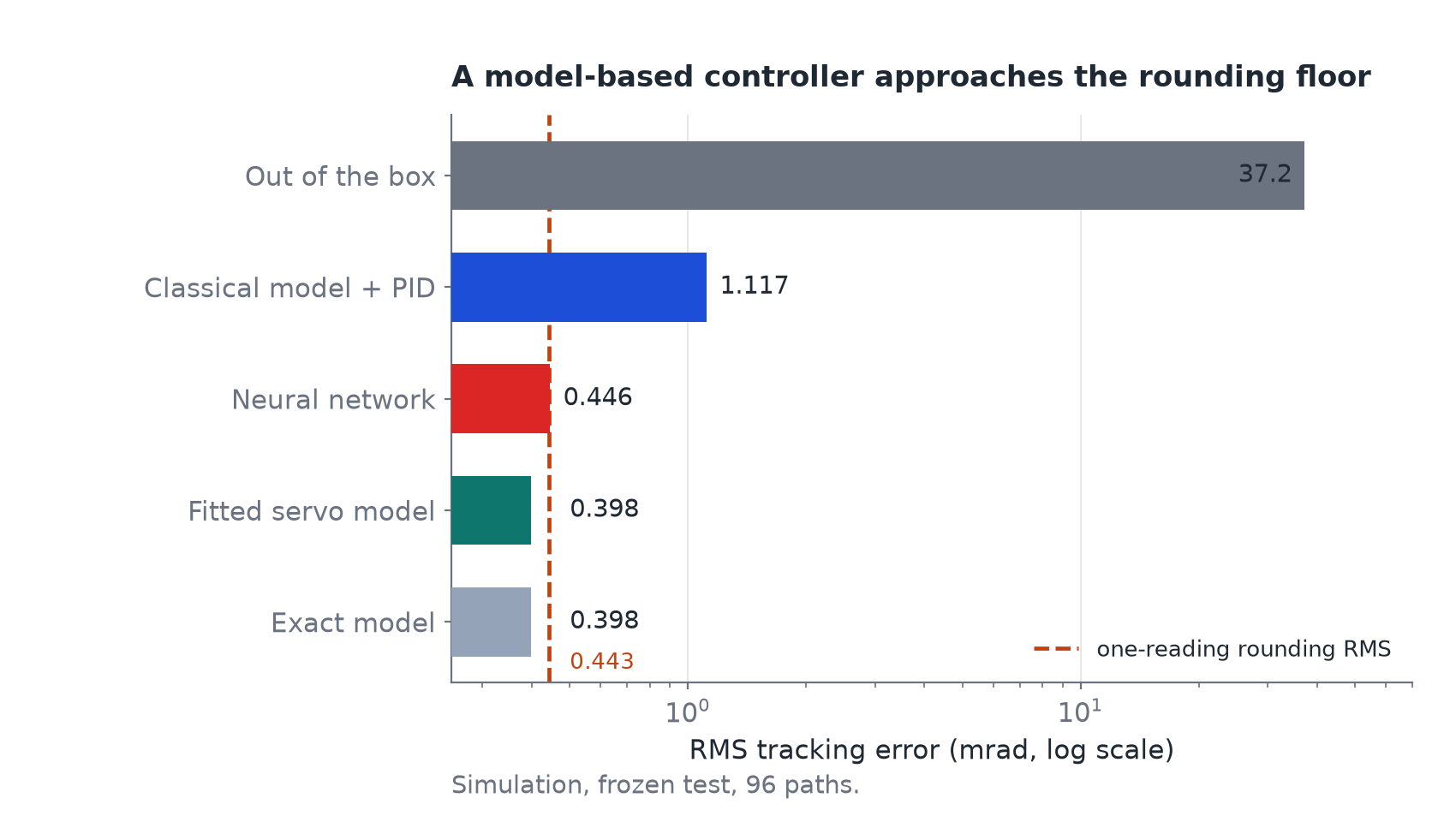
The simulation study compared these five controllers. All five read the same rounded encoder reading.

Controller	Family	How it chooses the goal	Error (mrad)
Out of the box	1	It sends the target as the goal, like `direct`.	37.2
Classical model + PID	3	It adds to the next target the torque that a fixed physics model predicts, divided by $k_p$ , then PI feedback.	1.117
Neural network	6	It adds to the next target an offset that a small network learned.	0.446
Fitted servo model	5	It simulates the next 33 ms step on a model fitted on 24 s of data, and solves for the goal.	0.398
Exact model	5	The same method as Fitted, with the true robot numbers.	0.398

Which error each controller removes, controller by controller

This matrix is the older view of the same information. Each row is a controller and each column is a kind of error, so if you see a particular error on your arm, you can read down its column.

Family 1: do nothing

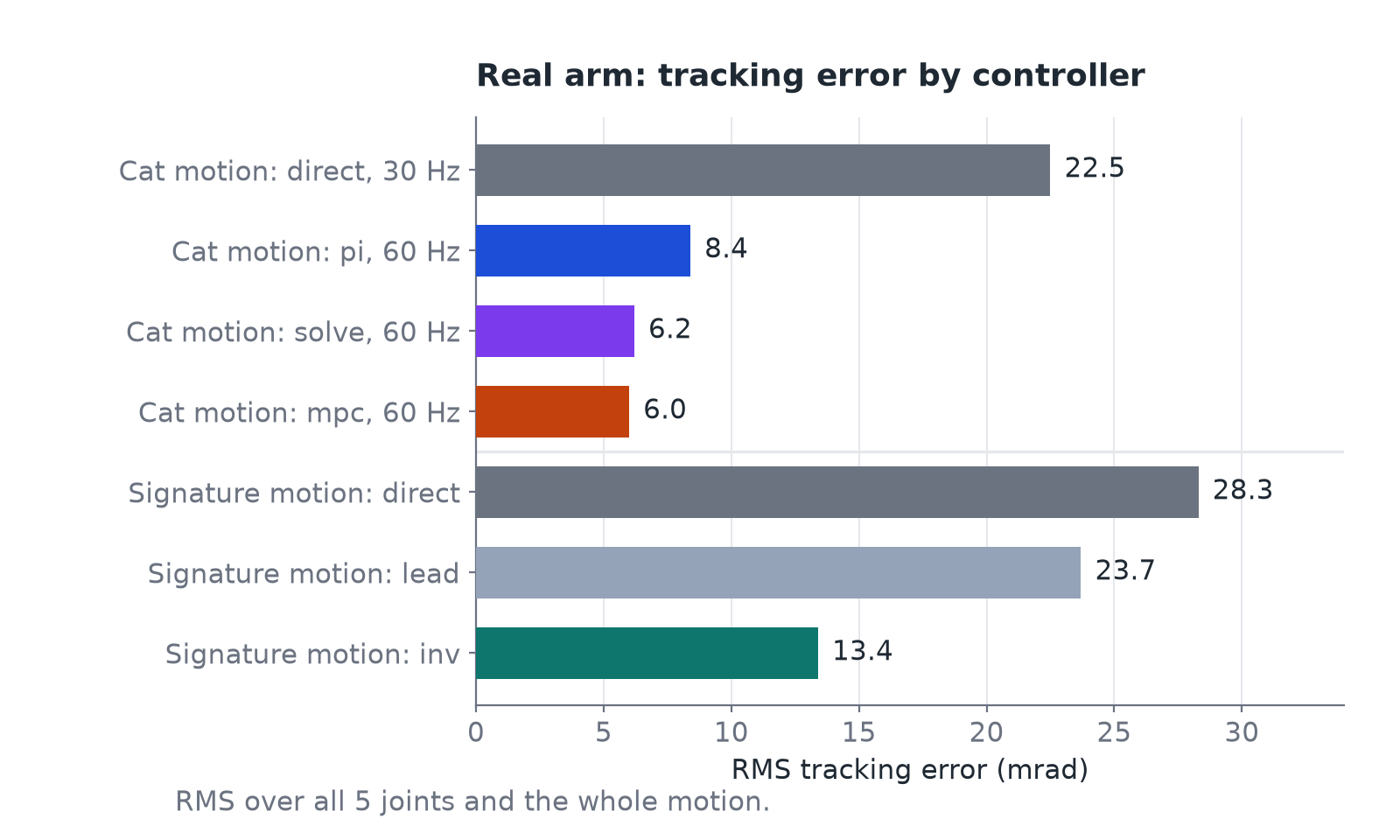
direct sends the target as the goal. Every term of the formula is zero. It's what LeRobot does, and on my real arm it gives 22.5 mrad on the cat motion at 30 Hz. All the other families are measured against it.

Family 2: look ahead in time

Problem: the goal acts late. The servo waits a dead time before it moves, the goal is held for a whole step, and wet friction adds a lag of $d/k_p$ .

Terms: $T$ , and the $\hat d$ and $\hat M$ terms that turn the lag into a time shift.

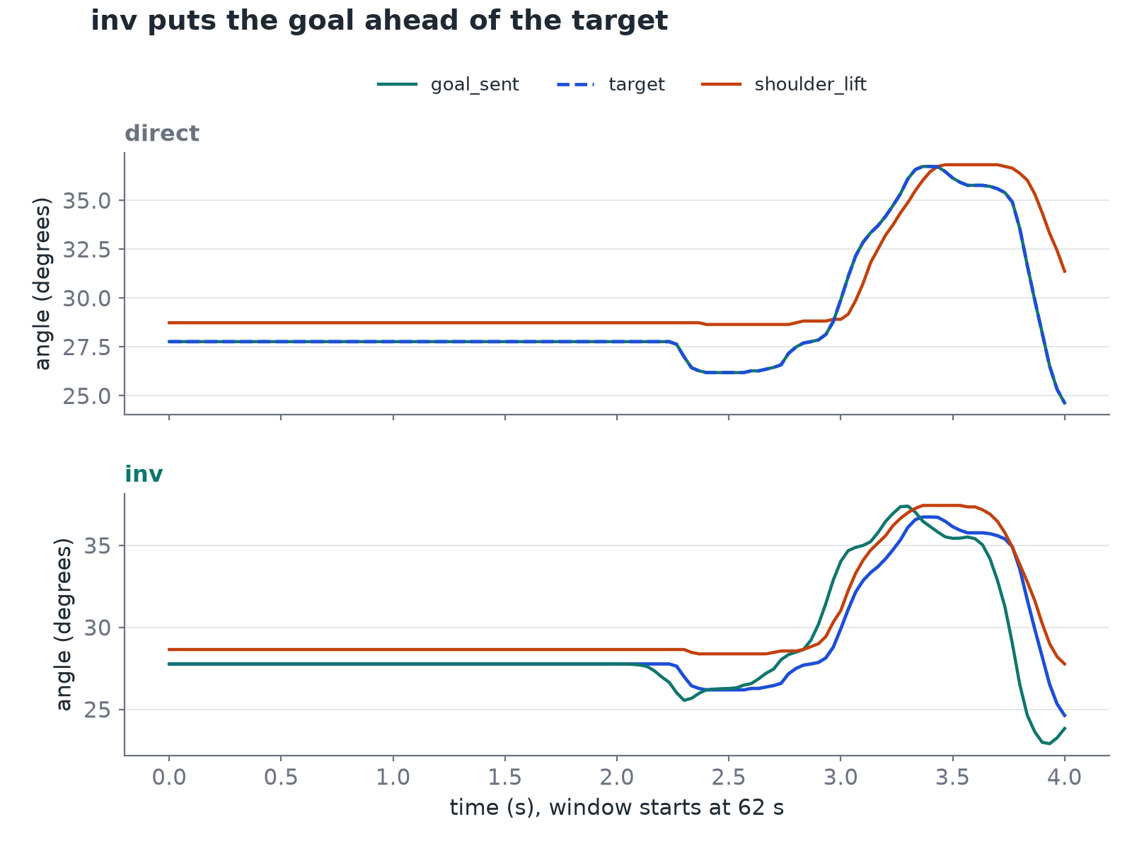
Two panels from the real arm on the same motion. With direct, the goal sits on the target and the joint arrives late. With inv, the goal leads the target and the joint lands closer to it. — Real arm, 30 Hz. `inv` sends the goal ahead of the target, so the joint arrives closer to on time.

Real arm on the same motion with `direct`, `lead` and `inv` at 30 Hz. The error is drawn 10 times larger, and large errors are compressed so the arm stays clear of the table and the base. The gray shape is the target pose. The red line joins the gripper tip to where the tip should be. The plot under each arm gives the true joint error in mrad, with the same scale in every plot. Open video

The simplest fixes don't look at the arm at all, only at the target. lead just sends the target one step early: $T$ = 33 ms at 30 Hz, and nothing else. inv goes further and inverts a simple model of the servo, with the dead time and the lag from the step test on my arm:

\text{goal}(t) = q^*(t + 33\ \text{ms}) + 0.106\ \text{s}\cdot\dot q^*(t) + 0.0023\ \text{s}^2\cdot\ddot q^*(t)

In the general formula, that's $T$ = 33 ms, $\hat d/k_p$ = 0.106 s and $\hat M/k_p$ = 0.0023 s². The second term is the wet-friction lag of part 1, and 0.106 s is close to the 87 to 105 ms lag of my real servo. The third term isn't computed from the masses of the arm: it's a coefficient fitted on the same step test, so it also absorbs whatever else makes the servo slow to accelerate. With a fitted constants file, each joint uses its own dead time, lag and acceleration term instead.

On the real arm, on a motion I call the signature, direct gave 28.3 mrad, lead 23.7 and inv 13.4.

This is feedforward: the goal comes from what I know about the target and the servo, not from the error. It's also the only thing that can deal with dead time, since any feedback arrives at least one dead time late. And because inv takes the speed and acceleration from the planned path, it doesn't suffer from the derivative noise of part 2. What it doesn't have is a gravity term, so the steady sag stays.

Is a fixed goal offset enough for the dead band?

Almost, with one change: the offset has to follow the direction. To push up you add the band, and to push down you subtract it. The trouble is near zero speed, where the sign flips, so the goal jumps by twice the band and can zig-zag. A smooth ramp near zero helps. A model that simulates the band handles the sign, the size and the dynamics together, which is one of the reasons for the planners of family 5.

Family 3: add the forces you know

Problem: forces that I can compute before the run, with a model of the arm: mostly gravity, and in simulation also inertia and friction.

Terms: $\hat G$ , and in the full version all of $\hat\tau/k_p$ .

sag and grav add a gravity term to inv. They differ only in where $\hat G$ comes from. sag fits it on steady holds of my real arm, using the sines and cosines of the link angles from part 1. grav computes it from a MuJoCo model of the arm at the target pose, divided by the stiffness. Both put in the gap that gravity needs ahead of time, so the joint doesn't have to sag into it. On my 3 Oct logs, friction hid the pose effect, so the fitted sag model came out almost as a constant offset for each joint.

The full version of this family is computed-torque control: compute every term of $\hat\tau$ from a physics model and add $\hat\tau/k_p$ to the goal. In the simulation study, Classical model + PID did that with the nominal robot numbers (inertia, gravity, damping and friction), plus PI feedback, and went from 37.2 mrad out of the box to 1.117. A version I call preview did the same with the MuJoCo inverse dynamics of the planned path, and I used it in the shake test of family 4.

The known forces did most of the work in both cases. Part of what was left came from how Classical uses its model, and family 5 explains that.

Family 4: estimate what you don't know

Problem: forces that no model knows before the run: a tool in the gripper, a worn joint, a simulator that is wrong about my arm.

Terms: $K_P$ , $K_I$ and $\hat w$ .

Feedback: pi

pi adds an outer PI loop on top of inv. It looks at the error $e$ , the target minus the reading, and moves the goal a little:

\text{goal} = \text{goal}_{inv} + 0.2\,e + 2\ \text{s}^{-1}\textstyle\int e\,dt

On the real arm the gains are small on purpose: 0.2 for the proportional part and 2 per second for the integral, with limits on both. The integral is the part that matters, because it slowly builds up whatever offset the model is missing, like a steady sag, until it's gone. On the cat motion at 60 Hz, pi gets 8.4 mrad. pisag is the same feedback on top of sag.

The gains are small because of everything from part 1. The arm only covers about 0.15 of a goal change in one 33 ms step, and the dead time means the loop always acts on old information. In the simulation study, the Classical controller used a much larger proportional gain of 4, without any dead time, and that's where I learned the next lesson.

The servo gap split into three parts: e from the servo spring, 4e from the outer loop, and the model offset, adding up to 5e plus the offset. — With an outer gain of 4, the joint feels 5 times the servo stiffness against a missing torque.

Predict first. A 150 g tool in the gripper needs 0.378 N·m of torque on shoulder_lift that the controller's model does not know. The controller adds an outer P term: it moves the goal by 4 × e, where e is the error (target minus reading). The servo stiffness is kp = 13.64 N·m/rad. Ignore friction and any integral term. What error stays? Pick the answer and its reasoning. (A) 27.7 mrad. 0.378 / 13.64. The outer P term does not change the servo. (B) 6.9 mrad. 0.378 / (4 × 13.64) = 0.378 / 54.6. The outer gain of 4 makes the joint 4 times stiffer. (C) 5.5 mrad. The gap is e + 4 × e = 5 × e, so the stiffness is 5 × 13.64 = 68.2 N·m/rad, and 0.378 / 68.2 = 5.5 mrad. (D) 0 mrad. Feedback removes any steady error. Answer: 5.5 mrad. The gap is e + 4 × e = 5 × e, so the stiffness is 5 × 13.64 = 68.2 N·m/rad, and 0.378 / 68.2 = 5.5 mrad.

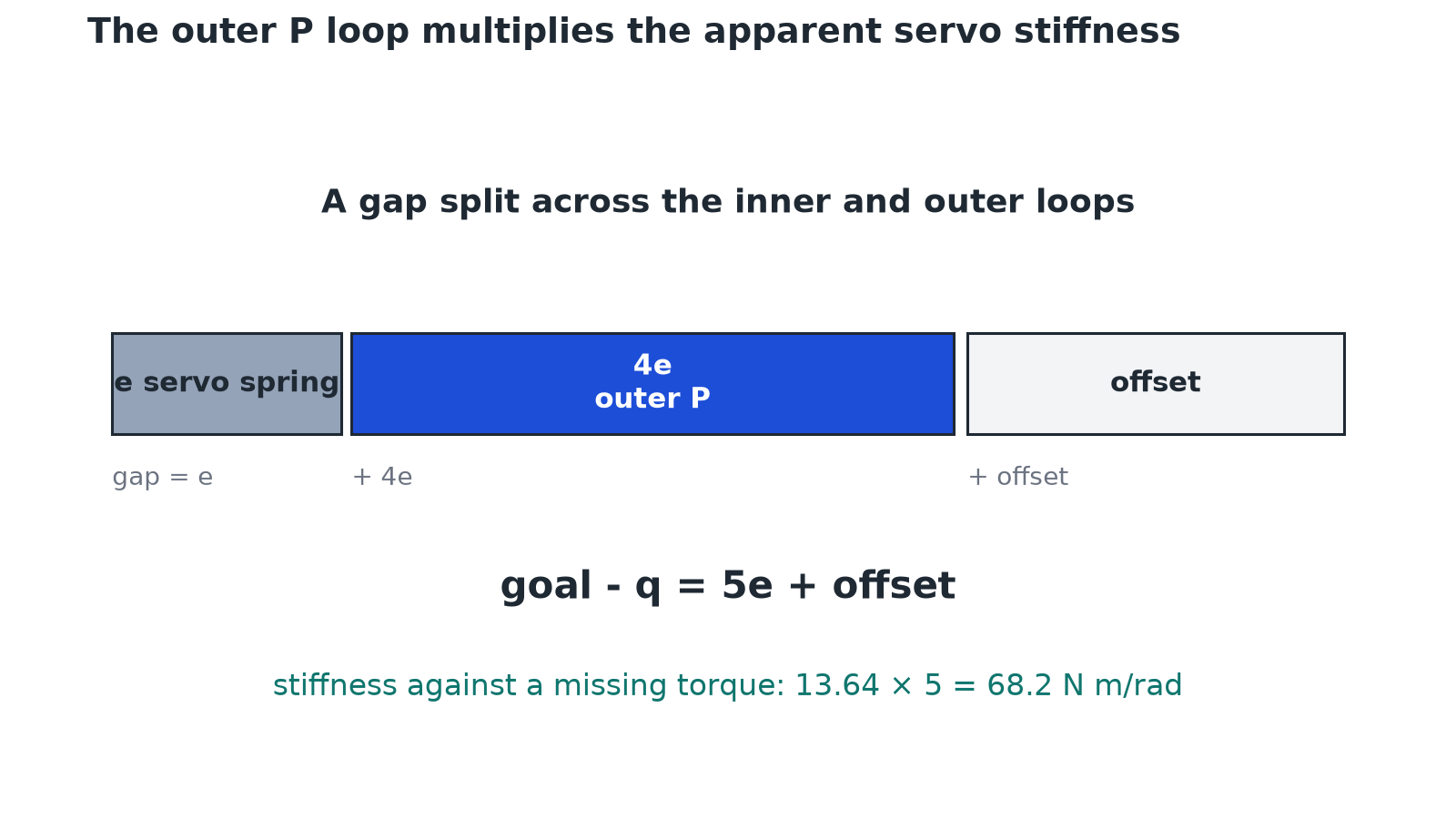
I assumed an outer gain of 4 would make the joint 4 times stiffer. It's 5 times. The servo gap is the goal minus the joint, which works out to

\text{goal} - q = (\text{target} - q) + \text{offset} + 4e = 5e + \text{offset}

The extra 1 is the servo spring itself. The goal already sits on the target, so a joint that's $e$ behind already has a gap of $e$ , and the outer loop adds 4 more on top. Against a missing torque, the stiffness is then 13.64 × 5 = 68.2 N·m/rad.

Where I was wrong: kp × 4

I multiplied $k_p$ by 4 and got about 7 mrad. I found the mistake myself after a while: I'd left out the servo spring.

Why not a gain of 100?

With a gain of 4, the arm covers about 0.6 of the error per step, which is stable. With a gain of 100 it would try to cover 15 times the error, so it overshoots, the next error is larger on the other side, and the oscillation keeps growing. A gain of 100 would also turn a single tick of reading noise into a 153 mrad jump of the goal. Add a 33 ms dead time and even a gain of 4 is too much: when I tried the Classical gains (4 and 10) with the dead time of my real arm in the shake test below, the servo spent about 95 % of the time at its torque limit.

The model also helps the feedback. A plain outer PID with no model saturated the servo on 10.9 % of the steps on a stiff simulated robot, while the same feedback on top of a model offset saturated on 0 %. The model does most of the work, so the feedback gains can stay low.

Shaking a load up and down, or left and right

This is the example that made the difference between families 3 and 4 click for me. Suppose I hold a weight in the gripper and shake it up and down. Gravity on the weight is a steady extra load, so the integral of pi should slowly build up the extra torque and hold it. Now suppose I shake it left and right instead. Gravity on the weight doesn't change, but the weight has to be stopped and turned around at each end of the stroke, and that inertia torque reverses every half stroke, so the integral is always half a cycle late. What should help there is something that sees the end of the stroke coming and starts pushing before it gets there.

I tested this in simulation, with the SO-101 model in MuJoCo, a 150 g load in the gripper, the simulated servo, a 33 ms dead time and a 30 Hz loop. The arm reaches forward and either the shoulder lifts the load up and down, or the base swings it left and right, by 0.1 rad at 1 Hz. I compared five controllers: direct, pi with the real-arm gains, inv plus pi, and two preview controllers from family 3, one with a model that doesn't know about the load and one that does.

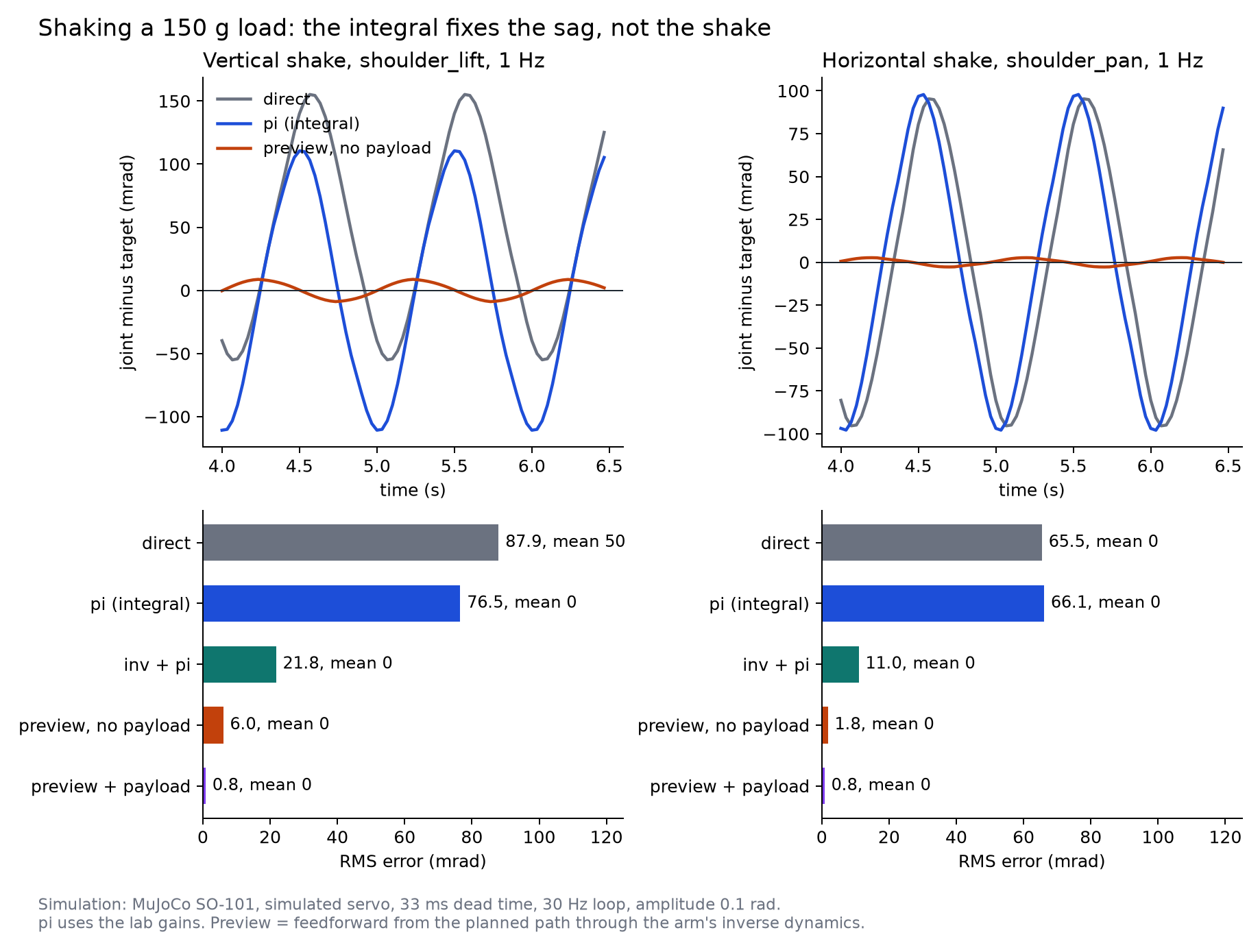
Two panels of error over time and two bar charts. In the vertical shake, direct has an error of 88 mrad with a mean of 50, pi has 77 with a mean of 0, and preview without the payload has 6. In the horizontal shake, direct has 65, pi has 66, and preview without the payload has 1.8. — Simulation. The integral removes the steady sag of the vertical shake but not the shake itself, and it does nothing for the horizontal shake.

Simulated SO-101 shaking a 150 g load at 1 Hz, error drawn 10 times larger. Top row vertical (plot: shoulder_lift), bottom row horizontal (plot: shoulder_pan); left `pi`, right preview. The four plots use the same scale. Open video

The result was half what I expected. In the vertical shake, the integral did remove the steady part: the mean error went from 50 mrad with direct to 0 with pi. But the shake itself stayed, with an RMS error of 77 mrad against 88, because the vertical shake also has to accelerate and stop the load, and that part reverses just like in the horizontal case. In the horizontal shake there was no steady part to remove, and pi did nothing at all, 66 mrad against 65.

What fixed both was looking ahead. inv plus pi brought the errors down to 22 and 11 mrad, and the preview controller to 6 and 1.8 mrad, even with a model that didn't know about the load. With the load in its model, both went under 1 mrad. So the integral handles what stays the same, and the path ahead handles what changes. In the formula: $K_I$ fills the constant part, and $T$ with $\hat M\ddot q^*$ fills the part that changes.

I didn't push this test hard enough to reach the torque limit, so the second half of my idea, that braking early is the only way to stop a heavy load in time, is still untested here. I also used a simple preview feedforward rather than the full mpc, so this shows what the path ahead is worth, not how well mpc itself uses it.

Better estimators: adapt and rls

The integral treats every missing force as one constant. The other two controllers in this family estimate more.

adapt keeps the plain inv goal and subtracts a $\hat w$ from a Kalman filter for each joint. The filter compares the angle that a fixed servo model predicts with the reading, and splits the difference into three parts: a fast load part, a slow sag part and a friction part. Part 2 explains the Kalman filter.

rls goes one step further: it changes the coefficients themselves during the run. It starts from the fitted servo model and updates a small linear model of the last two positions and goals with recursive least squares, forgetting old data slowly, then picks the goal that makes that model reach the target.

Family 5: plan with a servo model

Problem: the parts of the servo with no formula inverse. The dead band makes the right goal jump when the motion reverses. The ticks make the goal a whole number. The goal hold means the goal acts for a whole step, not an instant. The torque limit means some motions need braking to start early.

Terms: the same as families 2 to 4, but the goal comes from a search on a simulated servo, not from a sum.

One instant is not one step

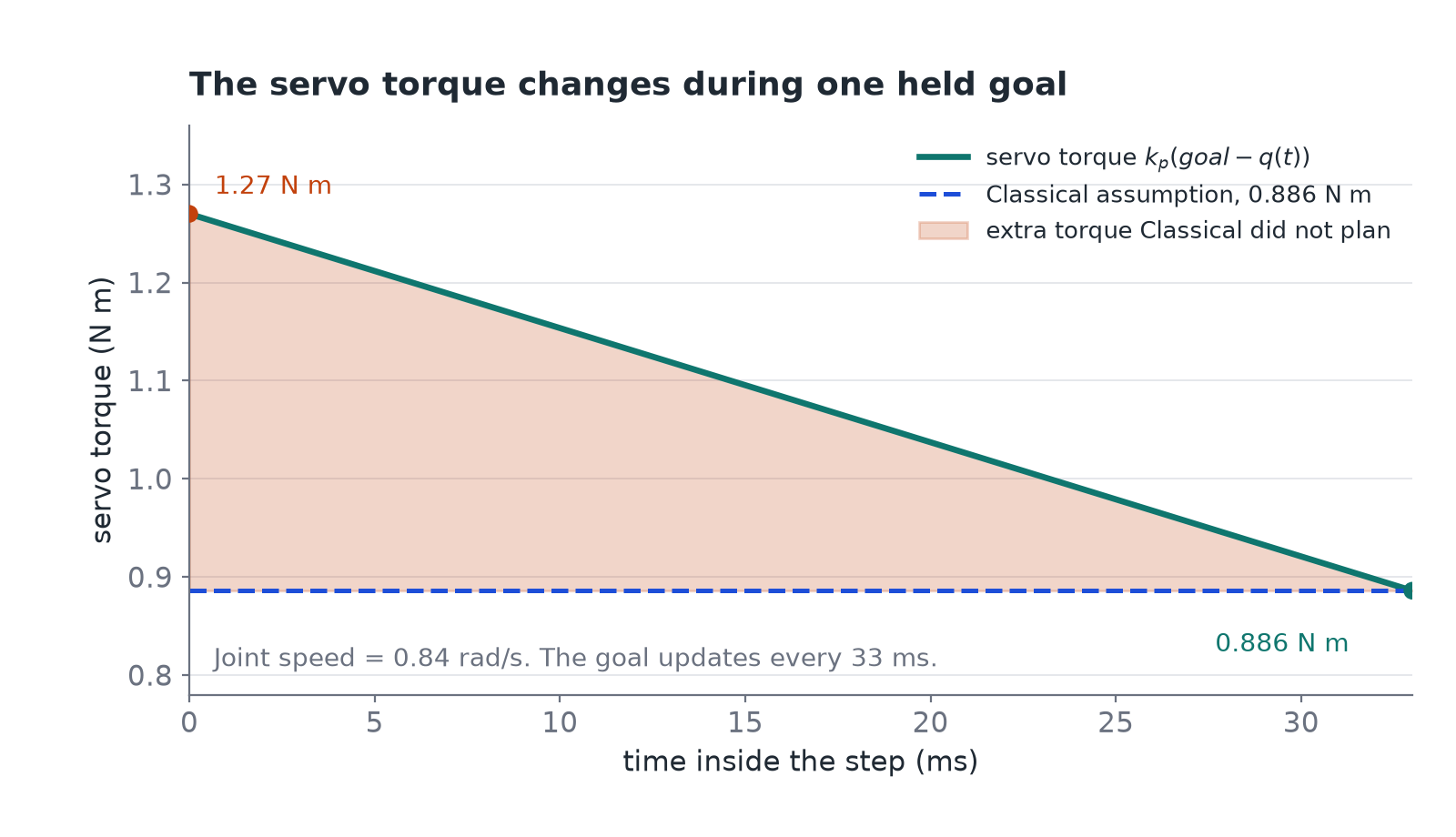
Servo torque during one 33 ms step at 0.84 rad/s. The real torque starts at 1.27 N·m and falls to 0.886 N·m at the end of the step. Classical assumes 0.886 N·m for the whole step. — Classical gets the torque right only at the end of the step. The shaded part is torque it did not plan.

The result that puzzled me first in the simulation study was that Classical loses to the Fitted servo model, even though it has a correct physics model of the simulated robot. The reason is how it uses that model. Classical picks the goal so that the torque is right at a single instant: it solves $k_p(\text{goal} - q) = \tau$ for the next target. But the servo holds that goal for a whole 33 ms step, and the arm keeps moving during the step. At the start of the step the joint is further behind, so the gap and the torque are larger than Classical assumed, and only by the end of the step are they about right.

Fitted gets around this by simulating the step in 8 small substeps and solving for the goal that puts the joint on the target at the end of the step, with Newton's method. Even with the true robot numbers, Classical's one-instant rule is still 3.4 times worse. A simple test made the cause clearer for me: the same Classical rule gets 4.13 mrad with a 30 Hz goal rate and 0.91 mrad at 240 Hz, so when the steps get shorter, the one-instant mistake mostly goes away.

Predict first. Give Classical model + PID the true robot numbers. Its error, averaged over six simulated robots, is 1.312 mrad. The Exact model has the same numbers and gets 0.385 mrad: it simulates the 8 substeps of each 33 ms step. Each controller uses its own tuned gains. A MuJoCo test changed one factor at a time. Which cause of the 3.4 times gap does it support best? (A) Its tanh friction model is wrong. (B) Its physics numbers are wrong. (C) It has no D term, so it cannot damp the arm. (D) Its rule treats the 33 ms goal hold as one instant. Answer: Its rule treats the 33 ms goal hold as one instant.

So I started to think of it as a ladder. Classical looks at one instant, Fitted simulates one step from the inside, and solve and mpc look many steps ahead. A trajectory is continuous, and each rung of the ladder sees more of it.

Where I was wrong: does the exact model see the true angle?

I thought "Exact" meant the controller got the true joint angle. It doesn't. It reads the same rounded reading as everyone else, and only gets the true robot numbers (supply, damping, friction, payload) once, when it's built. It has the same eyes as the others, just a better instruction manual.

Why Fitted's cost has a speed term

Fitted's cost is

J = |q_1 - r_{k+1}|^2 + (0.5\,\Delta t)^2\,|v_1 - \dot r_{k+1}|^2

The first part asks whether the joint reaches the next target at the end of the 33 ms step, and the second asks whether it moves at the target speed when it arrives. Two goals can put the arm on the same point, one with the arm still and one with it still moving fast, and the fast arrival overshoots in the next step. The factor $(0.5\,\Delta t)^2$ turns a speed error into a position error: $0.5\,\Delta t$ = 16.7 ms, so 0.1 rad/s counts like 1.7 mrad. In simulation, a speed weight of 0.25 gave 0.516 mrad, 0.5 gave 0.396, 1.0 gave 0.528 and 2.0 gave 1.556. The lab mpc doesn't need this term, because it plans 0.25 s ahead and sees the overshoot directly.

Planning many steps ahead: solve and mpc

This is the part I understood least, so I'll go slowly. On the real arm, both planners do the same thing at each step:

Take the current reading and the target path for the next 0.25 s.
Use a model of the servo to predict where the joint will go for a given plan of goals.
Pick the plan with the smallest predicted error.
Send only the first goal of that plan.
At the next step, plan again from the new reading.

That last part is called a receding horizon: the plan itself is never executed, only its first step. The 0.25 s look-ahead is about the dead time plus two servo lags, because a shorter one wouldn't see the effect of the goal I send now. The servo model has the dead time, the lag, the dead band, the stiffness and the sag of each joint, fitted on logs from my arm, plus a slow $\hat w$ that moves dt / 0.3 s of the way toward the unexplained error at each step.

The two planners differ only in the plans they can choose. solve chooses one number per joint, a destination goal on whole encoder ticks, and the goals in between follow a fixed rule toward that destination. So it searches a family of plans with a single knob. mpc, model predictive control, chooses one goal for each step of the horizon, 8 goals at 30 Hz, 15 at 60 Hz and 25 at 100 Hz, so its plan can do anything: overshoot, brake early, or hold. Its cost has three parts: the mean squared tracking error, a small cost on goal changes beyond what inv would do, and a tiny cost on straying away from inv.

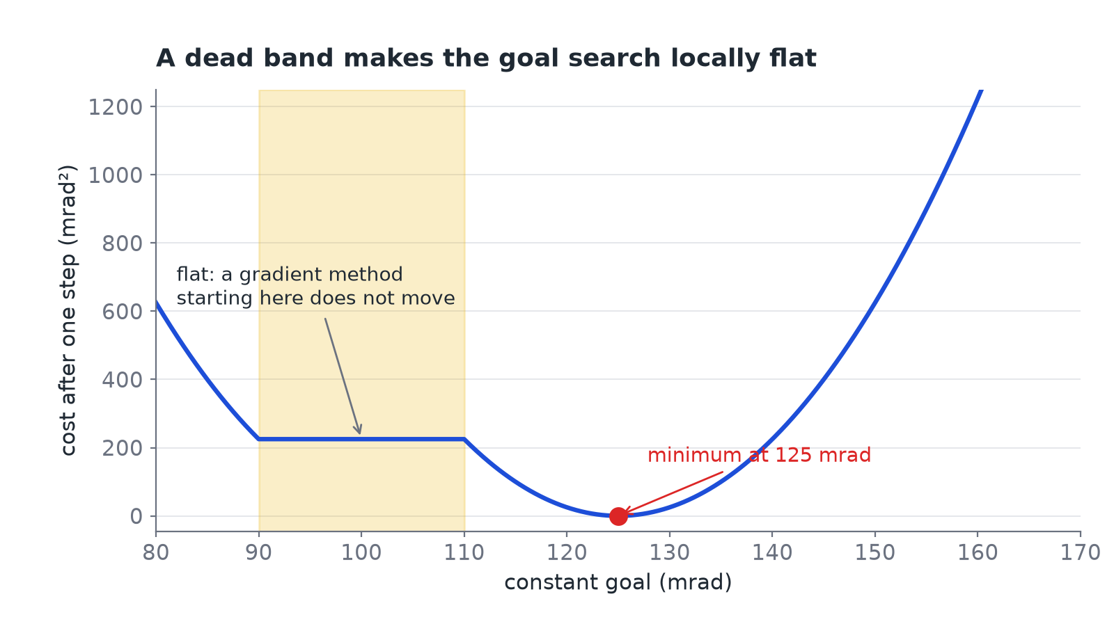
Cost after one step against a constant goal. The cost is flat from 90 to 110 mrad, inside the dead band, then falls to its minimum at 125 mrad and rises again. — The toy dead-band case: a gradient method that starts in the flat part has nothing to follow.

A toy example shows why a search is needed. Suppose the joint is at 100 mrad, the target is 115, and the dead band is 10 mrad on each side. Any goal between 90 and 110 makes no torque at all, so the joint stays at 100 and the error stays at 15. Above 110, the joint follows the goal minus 10. If you plot the cost against the goal, it's flat from 90 to 110 and then falls. A gradient method that starts somewhere in the flat part sees a slope of zero and doesn't move. solve avoids this by trying a list of whole-tick destinations directly.

How mpc gets out of the flat part: 50 warm starts

mpc starts from 50 different plans: 49 plans of the form "inv plus a constant offset", spread across the band, plus the previous step's plan shifted by one step. Then it takes two Gauss-Newton steps from the best one.

Two rules against chatter, and the reversal gate with numbers

Left alone, both planners chatter, and two rules fix most of it. The hold rule keeps the last goal if a new plan would gain less than half a tick, which stops the goal from flipping every time the reading flips between two ticks. The reversal gate deals with the dead band: a correction that reverses across the band costs a big goal jump, so the gate only allows it if it gains at least 1.5 ticks (2.3 mrad) and at least about 0.2 s have passed since the last reversal. Without the gate the goal reversed up to 17 times per second, and with it 1.8 times or fewer. The price is 0.4 to 1.0 mrad more error on holds.

Suppose the dead band is 10 mrad on each side and the last push was up: the goal is at 110 and the joint sits at 100. The target is 99. To move the joint down even 1 mrad, the goal has to drop below 90, a jump of more than 20 mrad. With a goal of 88, the joint goes to 98, now 1 below the target. To fix that, the goal has to go back above 108, another 20 mrad jump. Each small fix overshoots, so the goal bounces up and down. The gate only lets a goal reverse against its last push if the model predicts at least 1.5 ticks less error, and if the last reversal of that joint is at least about 0.2 s old. A reversal in the direction the target is moving is always allowed. The price is that a static error below about 1.5 ticks can stay.

Can they model gravity at different poses?

Partly. The servo model has the sag terms from the link angles, as in part 1. They're in goal units, radians of steady error, rather than in torque.

Why not run a full physics simulator inside?

I asked this too. They do simulate a model and keep the best goal, but the model is small: one fitted model per joint, from real logs. There are three reasons. The first is time: one 0.25 s MuJoCo rollout of the SO-101 takes about 0.75 ms on my Mac, the budget at 100 Hz is about 2 ms per step, and the planners test dozens of plans. The second is coupling: in the full arm, the shoulder goal changes the elbow load, so the search would have to try combinations of all five joints instead of five separate searches. The third is accuracy, which matters most. A physics model is only as good as its constants, and the masses in the model aren't measured on my arm. A Genesis model fitted to my arm predicted held-out logs only a little better than the small servo model (elbow 13.5 against 16.1 mrad, in simulation). So the real question isn't physics or no physics, it's which model predicts my arm best and fast enough.

Where I was wrong: is solve the same as Mink?

I thought solve was basically Mink. It isn't. Mink is inverse kinematics: it turns a gripper pose into joint motions from the geometry of the arm, it doesn't know about the servo, and it doesn't look ahead in time. solve comes after that step. The joint target is already known, and it chooses the servo goal over time.

On the real arm, on the cat motion at 60 Hz, the errors in mrad were:

Controller	Total	pan	lift	elbow	wrist flex	roll
pi	8.4	6.6	10.8	11.0	7.0	4.9
solve	6.2	3.2	7.4	6.7	8.7	2.8
mpc	6.0	3.0	7.0	6.1	8.6	2.8

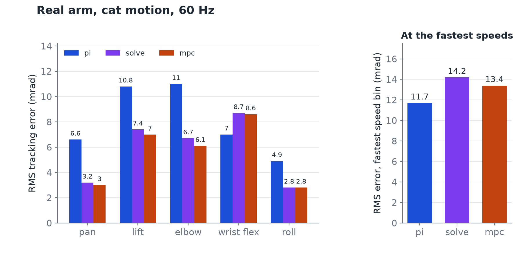
Left: RMS error per joint on the real arm for pi, solve and mpc. The planners win on pan, lift, elbow and roll, and lose on wrist flex. Right: at the fastest speeds pi has 11.7 mrad against 14.2 for solve and 13.4 for mpc. — Real arm, cat motion, 60 Hz. The planners win overall, and pi wins at the fastest speeds.

The planners win overall, but the picture changes with speed. On the fastest parts of the motions, pi does better, 11.7 mrad against 14.2 for solve and 13.4 for mpc. Most of that comes from wrist_flex, with 24.7 and 24.8 mrad for solve and mpc against 16.0 for pi. One possible cause is a step limit that the planners hit on 1 % to 3 % of the steps, but I haven't verified it, and each controller ran only once.

Planning with a better estimate: mpca

mpca is mpc with the Kalman estimate of adapt in place of its own slow $\hat w$ , so it combines families 4 and 5. In a simulated load step, mpca got 2.5 mrad against 3.7 for mpc at 30 Hz.

On my real arm, mpca is the controller I ran the most. On one 120 s motion at 60 Hz, with the fitted constants of my arm, it kept shoulder_lift at 10.3 mrad RMS. direct on the same motion and at the same rate gave 87.6 mrad, mostly because the arm reaches out and sags (mean error 70 mrad).

Real arm, same motion, 60 Hz: `direct` against `mpca`. The error is drawn 10 times larger, and large errors are compressed so the arm stays clear of the table and the base. The gray shape is the target pose. The red line joins the gripper tip to where the tip should be. The plot under each arm gives the true joint error in mrad, with the same scale in every plot. The plots cover the first 16 s; the RMS numbers in the text cover the whole 120 s run. Open video

Is mpca state of the art?

It's a strong classical baseline of a known type rather than a new method. MPC with an extra disturbance state estimated by a Kalman filter is a standard design, often called offset-free MPC.

Family 6: learn from repeats or data

Problem: errors that the other families leave because the model has the wrong form, or that come back each time the arm repeats a motion.

Terms: $u_k$ , or the whole $\hat\tau/k_p$ part learned by a network.

This family is where learning enters, and it gets its own article. Part 4 covers ilc and ilcmpc, the network of the simulation study, the result that changed how I test everything, and the idea I find most promising: a network that only learns what the physics misses.

Known territory

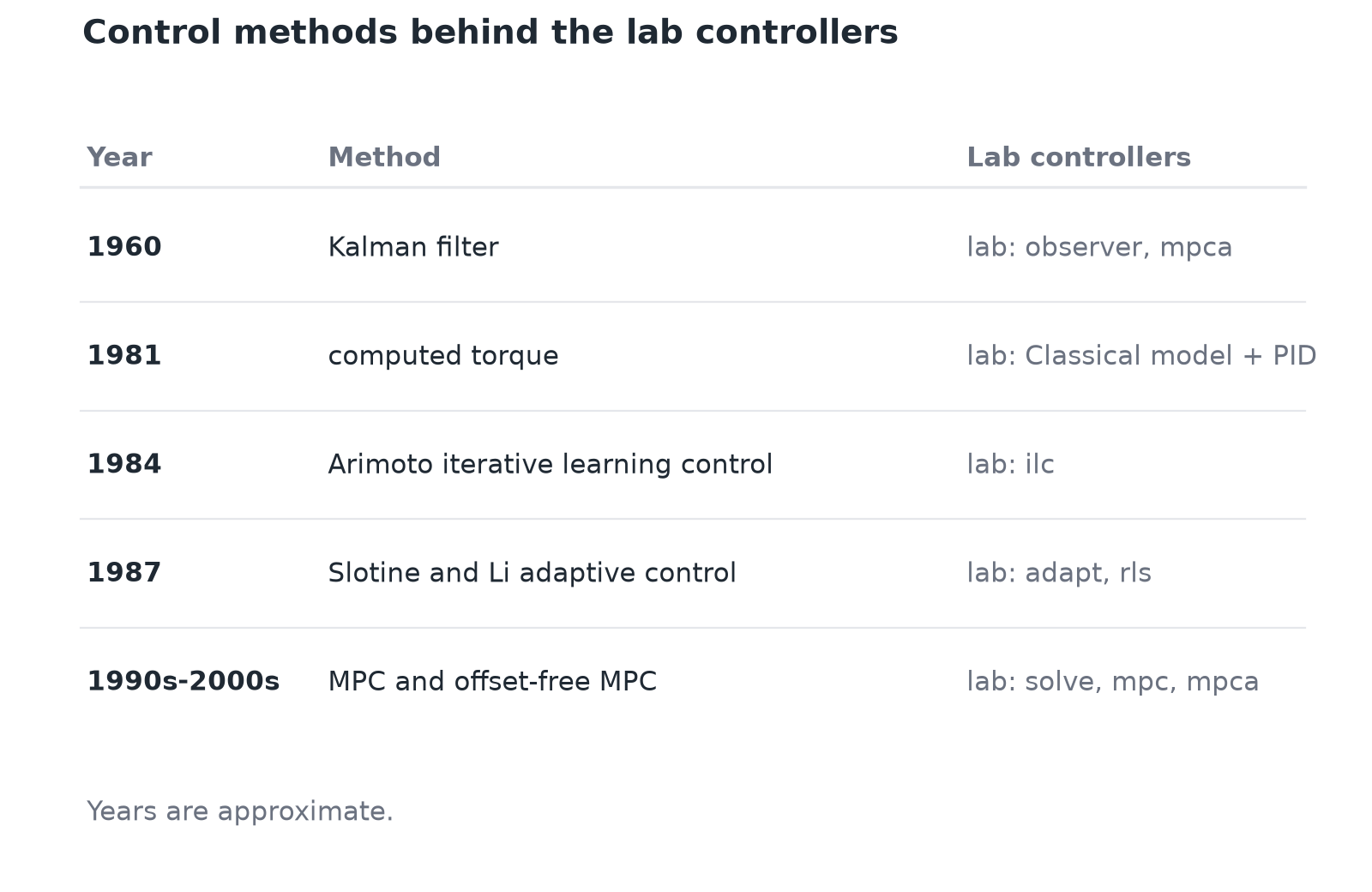
Timeline of the known control methods behind the lab controllers: the Kalman filter, computed torque, iterative learning control, adaptive control by Slotine and Li, and offset-free MPC. — Most of what I built has a name and a history.

Am I reinventing control? Mostly, yes, and I think that's fine for learning it. Each family has a name in the textbooks. Family 3 with feedback, Classical model + PID, is computed-torque control, inverse-dynamics feedforward plus feedback, from the 1980s. Estimating a payload during the run, family 4, is adaptive control, and since robot dynamics are linear in the mass parameters, a payload can be estimated online with a stability proof (Slotine and Li, 1987). mpca is offset-free MPC: a planner with a disturbance state estimated by a Kalman filter. And ilc is iterative learning control. What's still open for me is the real arm, and conditions that change during a task.

What's next

Every controller in families 1 to 5 uses a model that I either wrote down or fitted. Part 4 is about learning: from repeats of the same motion, from data with a network, and from both physics and a network together.

← All writing