Learning what the physics misses

Part 3 wrote every controller I built as one formula for the goal, and grouped them in six families. The first five families use a model that I wrote down or fitted. This part is about the sixth family, where the controller learns: from repeats of the same motion, from data with a neural network, and from both physics and a network together.

The question of the whole series was whether a controller can be more accurate than the classical ones. My answer at the end of this part: a network alone wasn't the way, but a network that only learns what the physics model misses is promising, and the research of 2026 goes the same way.

This part uses these controller names. Each one sends a position goal to the servo at each tick.

Name	What it sends to the servo as the goal	What it needs
`pi`	The target a little ahead in time, plus a correction from the recent error (proportional and integral feedback)	The target path and the reading
Classical model + PID	The target plus the torque of a fixed physics model divided by the servo stiffness, plus `pi`-style feedback	Nominal masses, friction and damping
`solve`, `mpc`	The goal that a servo model predicts will best follow the target over the next 0.25 s, found by search	A fitted servo model and the reading
`mpca`, `adapt`	Like `mpc` or `pi`, plus a Kalman filter that estimates a missing torque during the run	The same, plus the filter
Fitted	The goal that a fitted servo model predicts will land on the next target, with the 33 ms hold simulated in 8 small steps	A fitted servo model
`ilc`, `ilcmpc`	`pi`-style goals (or `mpc` goals), plus a correction learned from earlier runs of the same motion	Repeats of the same path
The network	A simple step rule plus an offset that a small neural network predicts	Recorded data
`phys`	The goal that a full physical model of the 5 joints predicts will best follow the target, found by search. An extended Kalman filter (EKF) estimates a missing torque $d$ for each joint	The full physical model, fitted on my real arm
PhysR	`phys`, with a small recurrent network that adds a learned torque inside the physical model	The same, plus recorded data

Family 6 in the formula

Problem: errors that the other families leave because the model has the wrong form, or that come back each time the arm repeats a motion.

Terms: $u_k$ , or the whole $\hat\tau/k_p$ part learned by a network, or a learned term added inside the physics model.

Learning from repeats: ilc and ilcmpc

If the arm does the same motion over and over, it can learn from its own past runs. Iterative learning control (ilc) stores the error of the last run and uses it to correct the goals of the next one: after each run, $u_k$ adds half of the error that step $k$ caused one servo delay later, then goes through a smoothing filter. ilcmpc puts that rule on top of mpc. In a stand-in test (a software copy of the servo, built from the servo model of my arm, which I use for dry runs) on the fast motion sets at 100 Hz, ilcmpc had the lowest error: 1.04 mrad, against 1.15 for mpc, 1.28 for mpca, 1.36 for solve, 4.15 for pi and 4.90 for adapt. The stand-in arm uses the same servo model as the planners, so this test favors them.

A network for the force terms

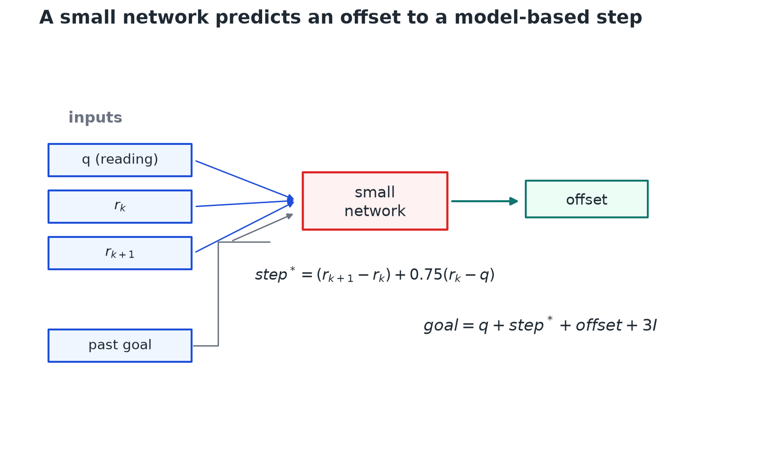
The question behind this whole series was whether a controller can be more accurate than the classical ones, so I also tried learning the goal with a neural network. In the general formula, the network fills the $\hat\tau/k_p$ slot: it doesn't output a goal from scratch, it outputs a correction on top of a simple rule,

\text{goal} = q + \text{step}^* + \text{offset}_{NN} + 3I

where $\text{step}^*$ is the move the controller wants this step: the target move, plus 0.75 of the distance the joint is behind.

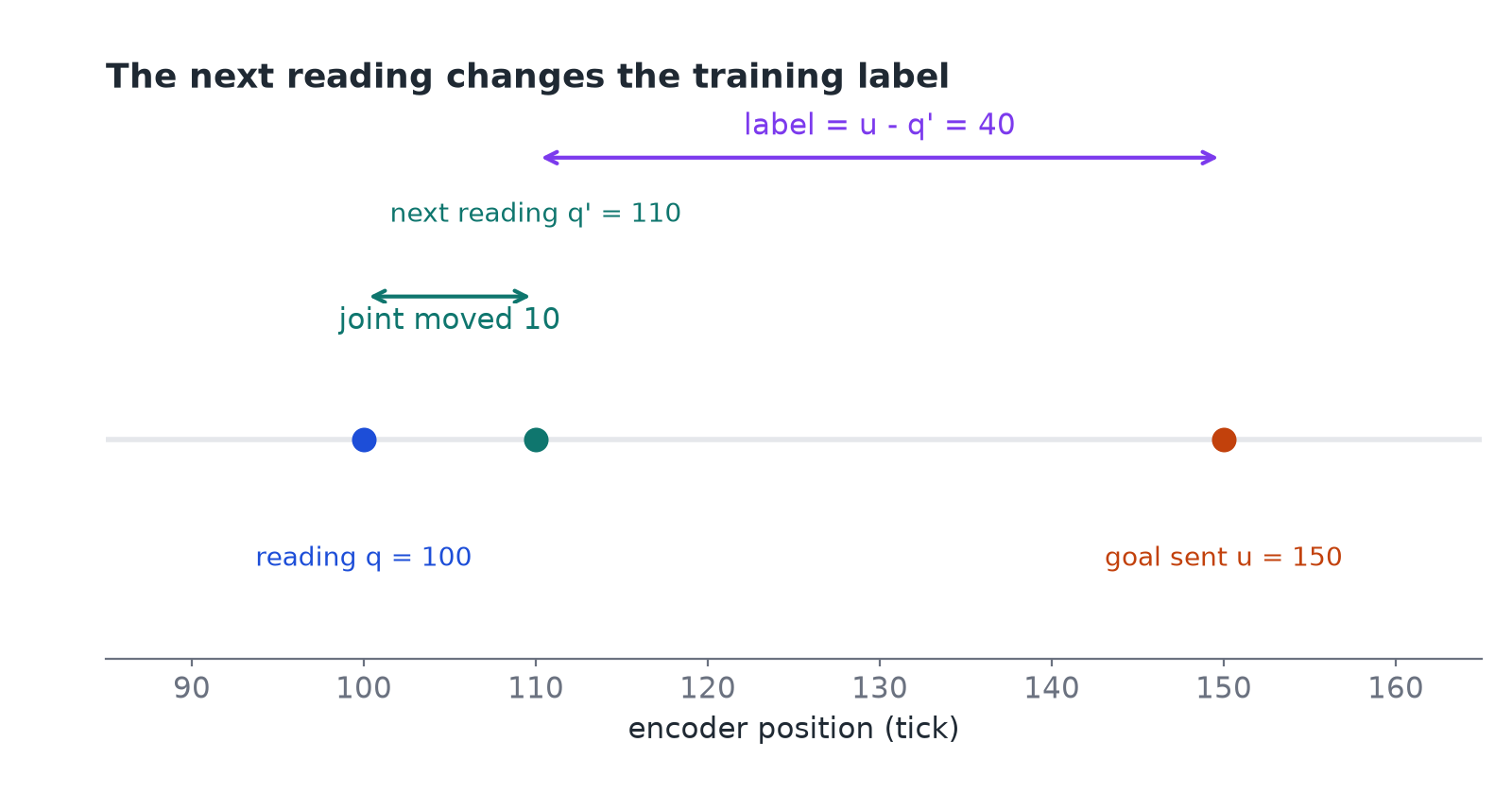
Number line in ticks: reading 100, next reading 110, goal sent 150. The joint moved 10 and the label, the goal minus the next reading, is 40. — The hindsight label: how far past the landing point the goal had to be.

Block diagram: the reading q, the targets r_k and r_k+1 and the past goal go into a small network, which outputs an offset. The goal is q plus step star plus the offset plus 3 I. — The network only learns an offset on top of a simple rule.

Its label comes from hindsight. Suppose a logged step where the reading was 100, the goal sent was 150 and the next reading was 110. The joint moved 10, and the goal sat 40 past where it ended up, so the label is 40. In words, the row teaches the network that from this state, to move 10, the goal has to go 40 past the end point.

The network has the same shape as Classical

$q + \text{step}^* = r_{k+1} - 0.25\,e$ . So Classical is $r_{k+1} + \tau/k_p + 4e + 10I$ , and the network is $r_{k+1} - 0.25e + \text{NN} + 3I$ . The network learns the part that Classical computes from physics, $\tau/k_p$ , and it learns it with the 33 ms step built in.

In the simulation study the network got 0.446 mrad, against 1.117 for Classical. That's because it learns the right lead for a goal that's held for a whole step, which is exactly what Classical's one-instant rule gets wrong. I first thought it was about knowing gravity in advance, but Classical knows gravity too.

Offline against closed loop

This is the result that changed how I test everything. There are two ways to test a network. Offline, you feed it recorded data and compare its output with the label, and its outputs never move anything. In closed loop, you let it drive the arm, so its goals move the arm and its next inputs come from that motion, including its own past goals.

Predict first. Two ways to test a network. Offline: feed it recorded data and compare its output with the label; its outputs never move the arm. Closed loop: let it drive the simulated arm; its goals move the arm, and its next inputs come from that motion, including its own past goals. Nominal = the default robot, with no change. An earlier network got 4 past readings and 4 past goals as extra inputs. It trained on smooth wiggle data only. Its offline label error fell from 6.19 to 3.03 mrad. In closed loop on nominal validation paths, the same network with no history had 0.552x the tracking error of Classical model + PID. Predict the closed-loop error of the network with history on nominal, as a multiple of the error of Classical model + PID. Answer: About 80x: 81.3x Classical model + PID, with 77% of steps saturated.

The answer was 81.3 times worse than Classical, with 77 % of the steps hitting the torque clamp. The history had halved the network's offline error, and in closed loop it was a disaster.

The reason is that one of its inputs is its own past goal. In the training data, the past goals came from a different controller, so the network never saw its own goals. Once it drives, a small mistake changes its next input, that input is a bit outside the data it learned from, so the next output is a bit more wrong, and the errors build on each other. The data the network sees in closed loop isn't the data it was trained on, which is called distribution shift. There's also a second suspect from part 2: the past readings give the network a noisy acceleration estimate, which the loop can amplify. I didn't test that one.

What I took from this is that a model has to be chosen by its closed-loop error. Offline training is simpler to run and simpler to think about, but only the closed loop actually tests the controller. From then on, every model choice in the project used closed-loop runs on validation paths.

Memory wasn't useless, by the way. With broadband training data, a wiggle from 0.2 to 14 Hz, a network with memory had 0.834 of the error of the old no-memory network, while the same network without memory had 1.45. The final network keeps one past step.

Where I was wrong: Classical doesn't look ahead

I said Classical doesn't look ahead. It does look one step ahead, since it uses the next target, so its $T$ is one step. Its weakness is treating the 33 ms step as a single instant.

Where the network wins and loses

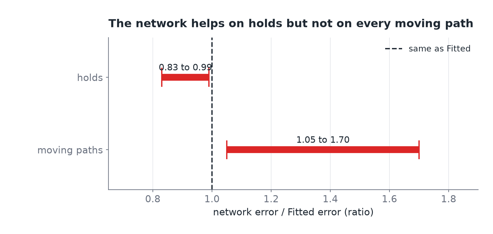
Network error divided by Fitted error: 0.83 to 0.99 on holds, below 1, and 1.05 to 1.70 on moving paths, above 1. — The network wins on holds and loses on moving paths. Simulation.

Compared with Fitted, the network wins on holds, with 0.83 to 0.99 of Fitted's error, and loses on moving paths, with 1.05 to 1.70. At a hold, the right goal is simple: the target plus a steady offset for gravity and friction. On a moving path, the goal has to sit far ahead of the joint, and the right lead depends on the speed, the acceleration and the 33 ms step. A model with the right structure gets that from physics, while the network has to learn it from data.

Is this overfitting?

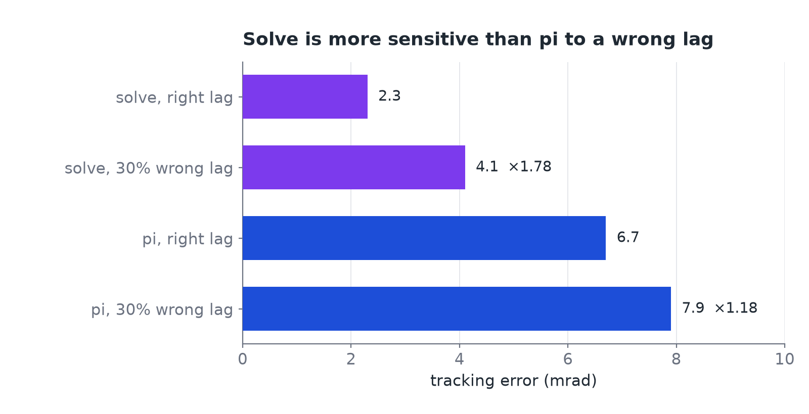
Tracking error with the right lag and with a 30 percent wrong lag: solve 2.3 then 4.1 mrad, 1.78 times worse; pi 6.7 then 7.9, 1.18 times worse. — A controller that trusts its model more loses more when the model is wrong, and still wins here.

I wondered whether a more complex physics model is simply more likely to be wrong, like overfitting. It's related, but the better name for it is sensitivity to model error. A controller that trusts its model more does better when the model is right and loses more when it's wrong. If I give solve a lag that's 30 % off, its error goes from 2.3 to 4.1 mrad, which is 1.78 times worse, while the same error only moves pi from 6.7 to 7.9, 1.18 times worse. Even with the wrong lag, though, solve is still better than pi. More terms aren't the problem in themselves, wrong terms are.

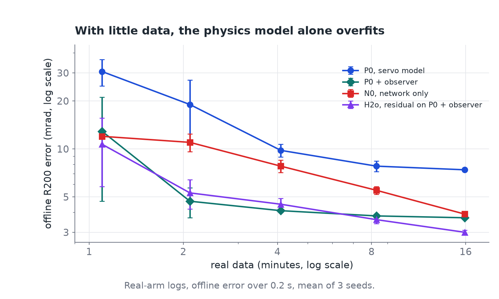
Real overfitting did show up once, with a physics model fitted on too little data. With 1 to 2 minutes of real data, the fitted servo model had 30.6 and 19.0 mrad of error on new motions, while a network with no physics had 12.0 and 11.0. The model's gain, offset and sag didn't transfer to new poses.

Offline error against minutes of real data, from 1 to 16 minutes. The servo model alone has 30.6 mrad at 1 minute and 19.0 at 2, falling to 7.4 at 16. With the observer it has 4.7 at 2 minutes and 3.7 at 16. The network alone falls from 12.0 to 3.9, and the residual from 10.7 to 3.0. — With 1 to 2 minutes of data the physics model alone overfits. The observer fixes most of it, and the residual is best with all the data.

A network that learns only what the physics misses

The network above learns the whole force term from data. The physics model of part 3 computes it from equations. A residual model does both: the physics computes what it can, and a network learns only the rest, the residual. In the joint equation of part 1, the residual $r$ is one more torque:

M(q)\ddot q + C(q,\dot q)\dot q + G(q) + d\,\dot q + f\,\text{sign}(\dot q) = k_p\big(\text{goal}(t-D) - \hat q\big) + \hat d + r_\theta(\text{history})

$\hat d$ is the missing torque that the Kalman filter estimates, and $r_\theta$ is a small recurrent network with weights $\theta$ . It reads the recent readings, goals and targets, and outputs a torque for each joint. The controller still chooses the goal by search through the whole model, so the network changes what the controller predicts, not what it sends. If the network learns nothing, the controller is the physics controller again.

Left: a frozen servo model with an observer plus a small recurrent network (GRU) that learns the residual give a combined prediction. Right: offline and stand-in closed-loop errors: network only 3.90 and 5.50 mrad, servo model with observer 3.70 and 2.76, residual 3.01 and 3.12. — First try: the residual helps offline, and the physics model alone still wins in the stand-in closed loop.

The same job as the Kalman disturbance

In part 2, the Kalman filter added a missing torque $d$ to the state of the joint. The residual does the same job. Both are a torque that the physics model misses, and both learn from the same signal: the prediction error, the reading minus what the model predicted.

The difference is what each one can express. The filter assumes that $d$ is constant, except for a small random step at each tick. So it follows a steady missing torque well, like a tool in the gripper. It is late when the missing torque changes as fast as the motion. The network computes $r$ from the recent history, so it can give a missing torque that depends on the speed, the direction or the pose.

Here is one example, with the teaching values of a single joint. The model says the damping is $b = 0.3$ N·m·s/rad, and the true damping is 50 % higher. The missing torque is then $-0.5\,b\,\dot q$ . At a steady 0.9 rad/s, it is $-0.5 \times 0.3 \times 0.9 = -0.135$ N·m, and the filter finds it. At a reversal to −0.9 rad/s, it jumps to +0.135 N·m. The filter still holds the old value, so its estimate is wrong by 0.27 N·m until the innovations pull it across. A network that sees the speed can give the new value at the reversal, if its training data had reversals like it.

This table compares the two on the same attributes.

	Kalman disturbance $\hat d$	Network residual $r_\theta$
What it is	One number for each joint	A function of the recent history
What changes during a run	$\hat d$ moves by $K_d$ times the prediction error at each tick	The memory (hidden state) of the network changes with each reading; the weights stay fixed
What teaches it	The prediction error of this run	The prediction error over many recorded runs, during training
What it follows well	A steady missing torque, for example a payload	A missing torque that depends on the state, for example damping or friction that changes at a reversal
Weak point	Late when the missing torque changes fast	Knows only the situations that the training data showed

The two also work together. In PhysR, the filter keeps estimating $\hat d$ during the run, and the network adds $r$ on top. The filter covers what the network never saw, like a new tool, and the network covers the fast, repeatable patterns that a constant can't follow.

What a position loss can't tell apart

My encoders measure angles, not torques. So the network learns its torque through the plant: the training compares the predicted angle with the measured angle, and the gradient goes back through the physics equations.

That has a trap. Take one joint at rest, with an inertia of 0.1 kg·m², and predict 0.1 s of motion under a constant torque. The angle changes by $\Delta t^2 \tau / 2I = 0.05\,\tau$ . The controller sends 0.6 N·m, and the joint moves only 0.02 rad. A missing torque of −0.2 N·m explains this: $0.05 \times 0.4 = 0.02$ . A larger inertia of 0.15 kg·m² explains it too: $0.01 / 0.3 \times 0.6 = 0.02$ . The data can't tell the two apart.

At a different command, the two explanations disagree. At 1.2 N·m, the torque explanation predicts 0.05 rad and the inertia explanation 0.04 rad. A search controller compares exactly such new commands. So a residual that predicts the logged commands well can still rank new commands badly. The logged commands are the commands of the old controller, not the commands the search tries. The residual is an effective term: it can absorb friction, delay, inertia and estimation errors, and it isn't a measurement of a physical torque.

What the residual gave so far

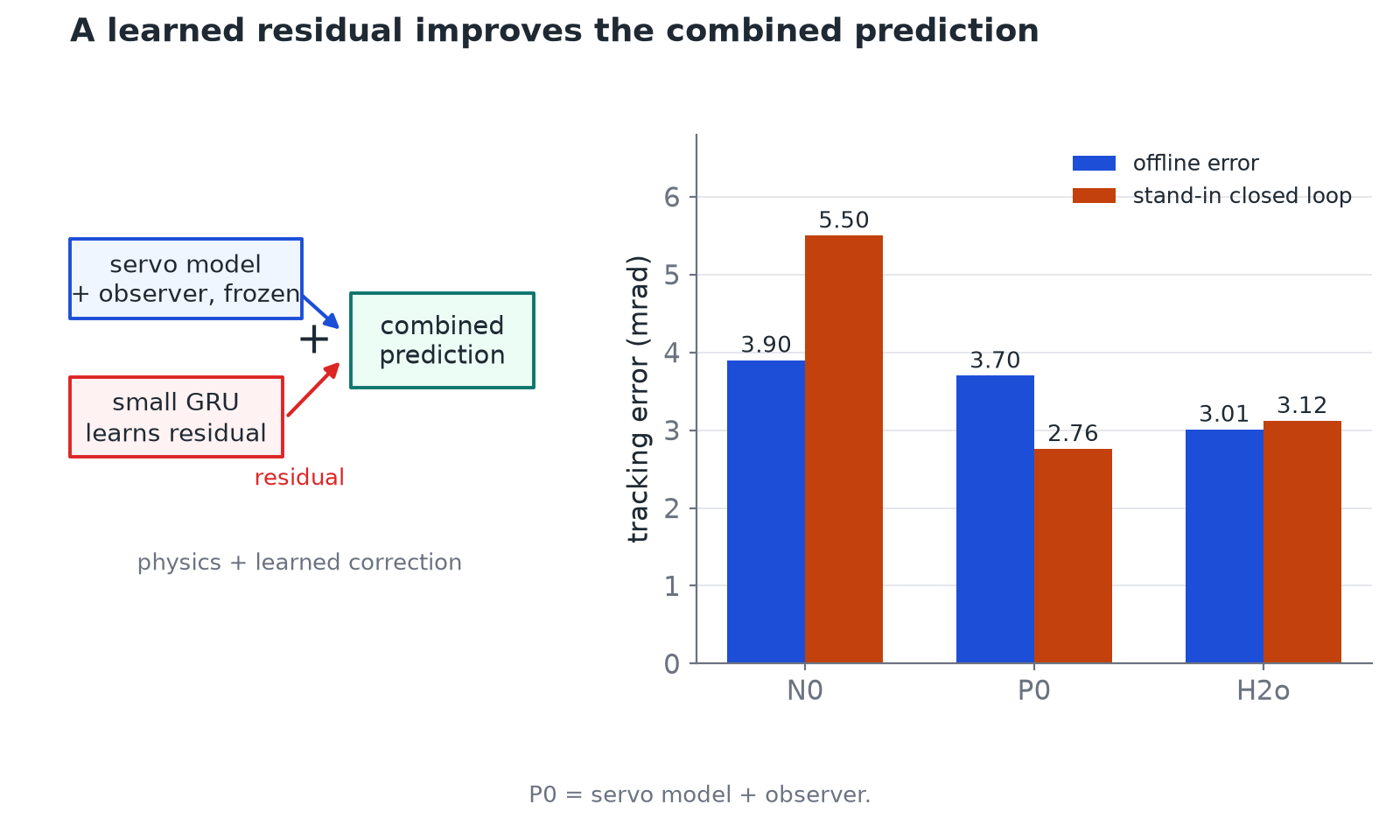
The first try put a residual on a simple servo model with an observer. It was measured offline over 0.2 s, and in a stand-in closed loop, a software copy of the servo model in place of the real arm:

Model	Offline (mrad)	Stand-in closed loop (mrad)
Network, no physics	3.90	5.50
Servo model + observer	3.70	2.76
Network residual on servo model + observer	3.01	3.12

Most of the gain is classical: the observer alone halves the servo model's error, from 7.37 to 3.70 mrad, and the residual adds another 19 % to 23 % offline. In the stand-in closed loop, the physics model alone still wins. The stand-in has the same structure as the servo model, so it favors it, and it doesn't tell me which one wins on the real arm.

The second try is PhysR, the residual inside the full physical model of phys. Its network is a GRU, a common type of recurrent network, with 64 units. It trained on real recorded windows, with the Kalman $\hat d$ held constant over each prediction. This table gives the error 6 ticks ahead (0.1 s at 60 Hz), on held-out real windows, offline.

Joint	Physics model alone (mrad)	PhysR (mrad)	Gain
shoulder_pan	2.92	2.70	7.5 %
shoulder_lift	4.78	4.19	12.3 %
elbow_flex	3.68	3.59	2.4 %
wrist_flex	2.21	2.03	8.1 %
wrist_roll	2.01	1.86	7.5 %

The gain is real and small: 2 to 12 % against the physics model alone. My first summary said 8 to 26 %, but that number compared PhysR with a constant $\hat d$ , which is worse than no $\hat d$ at all when the arm moves. All these numbers are offline, on windows that other controllers drove. No closed-loop PhysR result exists yet, and offline against closed loop showed why that matters.

What other research does

I wanted to know if this is a dead end or a direction other people take too. A short review of 2026 papers says it is a direction, with a twist: the useful comparison isn't which network is best. It is where each method puts the learning. A network can sit in four places: inside the model, after the controller on the command, before the controller on the reference, or above everything in the task policy.

This table places five recent papers and my own PhysR by where the learning sits.

Method	Where the learning sits	What it learns, and how	Hardware	Limit
NeuralActuator (RSS 2026)	Model	A Transformer gives an effort estimate to a differentiable simulator. Measured positions train it through the simulator, like my position loss	Includes SO-101 STS3215 servos	The offline rollouts use recorded future effort, which a new candidate goal doesn't have
PG-RSSNN (IFAC 2026)	Model	Physics state equations plus a recurrent correction, trained on the multi-step prediction error	KUKA arm, prediction from recorded torques	Prediction only; no control result
Energy-regularized neural MPC	Model, inside MPC	A learned acceleration correction that takes the candidate input, plus a penalty against corrections that break the energy model	Aerial robot, flight tests	It doesn't win on every path
OSRAM	Reference	Learns how the robot and its controller respond together, then adjusts the reference. The weights adapt after deployment	Tron1	The error summaries use only successful trials
TAM (CoRL 2026)	Command, after the controller	Adds a torque correction after the controller. A history encoder infers a context at about 5 Hz with fixed weights	Franka Panda, torque input	Needs a torque input and simulation teacher labels; the SO-101 takes position goals
PhysR (mine)	Model, inside a search controller	A GRU torque residual inside the full physical model, trained through the plant	SO-101, position goals	2 to 12 % offline; no closed-loop gain yet

Two more names come up often, RECAP and π0.7. They learn the task policy, the part that chooses the grasp or the next pose. That is a different level. A better grasp choice doesn't fix a servo that stops short, and a better servo model doesn't fix a bad grasp. A task policy could give the references that phys or PhysR executes.

The closest paper to my project is NeuralActuator. It uses the same servos and the same idea of a position loss through a simulator. PhysR differs in one main way: it keeps the explicit physics and learns a correction, while NeuralActuator predicts the effort directly. Energy-regularized neural MPC shows one thing PhysR doesn't do yet. Its correction takes the candidate command as an input, so the controller can rank different commands with different corrections. PhysR gives one correction that all candidate goals share.

Three meanings of adaptation

Papers often say their method adapts online. Suppose you put a 200 g tool in the gripper. Three different things can adapt, and this table separates them.

Mechanism	What changes	What stays fixed	Example
Recurrent inference	The memory of the network, from new readings	The weights	TAM context, the PhysR GRU state
Weight adaptation	The weights, from training on new data	The architecture	OSRAM after deployment
Classical estimation	An estimated state or parameter	The model structure	The Kalman $\hat d$ of `phys`, RLS

The Kalman filter of part 2 is the third kind. A recurrent residual is the first kind: it adapts in the same way, from each new reading, with no new training. If a change is outside what the training data showed, for example a payload heavier than any in the data, recurrent inference probably fails, and the Kalman $\hat d$ still follows it, because it has no learned range. This is one more reason to keep both.

How far each result goes

A result can support five claims, and each claim asks more than the one before it.

Prediction: the model reproduces held-out recorded motion.
Command choice: the model ranks alternative commands correctly.
Physical control: the controller reduces the tracking error on the real robot.
Adaptation: the controller keeps that gain after a specified change, like a new payload.
Task success: the gain helps the task the robot is for.

PhysR is at step 1, with a small gain. PG-RSSNN is at step 1 too. Energy-regularized neural MPC reaches step 3 in flight tests. Most claims of "a better model" stop at step 1, and offline against closed loop is my own example of how step 1 and step 3 can disagree.

What I test next

These are the tests that I think decide whether PhysR is worth it, each with my prediction.

Matched closed loop on the real arm. Run phys, phys with a better forecast of $\hat d$ , and PhysR, on the same motions, with the same timing and limits. Prediction: PhysR wins most near reversals, and a better $\hat d$ forecast gets part of that gain with no network.
A residual that depends on the candidate goal. Give the network the candidate goal as an input, like energy-regularized neural MPC. Prediction: it helps near reversals, the dead band and the torque limit, where different goals give different missing torques. The test is whether it ranks candidate goals in the same order as the measured responses.
Train on its own closed loop. Collect data with PhysR in the loop, train again, and repeat. Prediction: the gain grows over the first rounds, because the data then has the commands that the search actually tries.

In each test, I choose models by their closed-loop error on the real arm. That last rule is the one I'll keep from this whole series.

Looking back

When I started, I thought the arm missed because it was cheap. Now I'd say it misses because the servo can only make torque from a gap, and every term of the joint equation, from gravity to damping to a tool in the gripper, needs a bit more of that gap. Every controller in this series is a guess at that gap, written as the same formula with different terms switched on. The best ones look ahead: they know the path, they know the servo, and they put the goal where the joint will need it, before it needs it. Learning helps most when it fills in what the physics misses, and the only test that counts is the closed loop.

← All writing