Seeing finer than the sensor

Part 1 wrote one joint of my arm as an equation, and every term in it uses the true angle $q$ . My controllers never see $q$ . They see the reading $\hat q$ , in whole encoder ticks of 1.534 mrad. Two questions kept coming back while I worked on this side of the equation. What happens when a controller needs more than the angle, like the speed or the acceleration? And can a controller know the angle better than the sensor tells it?

Part 3 groups my controllers into six families. This part uses four of their names. This is what each name means.

Name	Family	What it sends to the servo as the goal	What it needs
`inv`	Look ahead in time	The target one servo dead time ahead, plus the target speed times the servo lag, plus a small acceleration term. It reverses a simple model of the servo, which is where the name comes from.	The dead time and the lag of the servo, from a step test on the arm.
`solve`	Plan with a servo model	A search for each joint. It tries many destination goals, simulates the servo model 0.25 s ahead for each one, and keeps the goal with the smallest predicted error.	The servo constants of the arm.
`mpc`	Plan with a servo model	Model predictive control. It uses the same model and look-ahead as `solve`, but it chooses a different goal for each step of the 0.25 s plan. It sends the first goal and makes a new plan at the next step.	The servo constants of the arm.
`mpca`	Plan with a servo model	`mpc` plus a Kalman filter that estimates a load and a sag during the run. The "a" means adaptive.	The servo constants of the arm.

The "servo constants" are a file with the dead time, the lag, the dead band, the stiffness and the sag of each joint, fitted on logs from my arm. Part 1 explains the dead time and the lag.

Ticks: the reading is rounded

The encoder doesn't give a continuous angle, it gives whole ticks, 4096 per turn, so one tick is 1.534 mrad. If the true angle is anywhere inside a tick, the reading is the same, which means there's a reading error underneath everything else the controller does.

How big is it on average? If the true angle is equally likely to be anywhere in the tick, the error is spread evenly from −0.5 to +0.5 tick, and its root mean square is

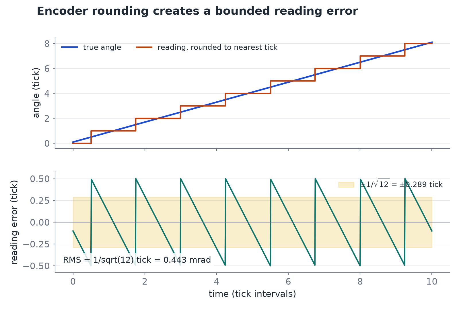
\sqrt{\int_{-1/2}^{1/2} e^2\,de} = \frac{1}{\sqrt{12}} \approx 0.289\ \text{tick} = 0.443\ \text{mrad}

Top: a ramp of true angles and the staircase of readings rounded to the nearest tick. Bottom: the reading error, a sawtooth between minus and plus half a tick, with an RMS of 1 over the square root of 12 tick, 0.443 mrad. — Rounding to whole ticks leaves a sawtooth error with an RMS of 0.289 tick.

Where I was wrong (half): the sqrt(1/3) step

When I tried this for an error spread from −1 to +1, I only got $\sqrt{1/3}$ after a hint to divide by the width of 2. Once I saw that, the same calculation over a width of 1 gave $1/\sqrt{12}$ .

I assumed this meant no controller could do better than about half a tick, but that's not quite right. The score measures the true angle, not the reading, and the joint doesn't jump between ticks: the spring, the damping and the inertia smooth its motion between two readings. Many readings together also carry more information than one, so a controller that uses them well can land closer than the tick suggests. That's what the rest of this part is about.

Two differences make a lot of noise

To push the arm along a path, you need to know how much torque it takes, and the equation of motion from part 1 needs the acceleration $\ddot q$ for that:

\tau = M(q)\,\ddot q + C(q,\dot q)\,\dot q + G(q)

A friend who works on robots told me that taking the acceleration from noisy encoder readings is a classic trap, and I wanted to see why with actual numbers. The simplest way to get the speed is from two readings, $v \approx (q_k - q_{k-1})/\Delta t$ , and the acceleration from three, $a \approx (q_k - 2q_{k-1} + q_{k-2})/\Delta t^2$ . Now suppose the reading is off by one tick. At 30 Hz, that one tick turns into an acceleration error of

\frac{1.534\ \text{mrad}}{(1/30\ \text{s})^2} \approx 1.4\ \text{rad/s}^2

which is about the same size as the real accelerations of a fast motion. What surprised me more is that it gets worse with a faster loop. The noise grows with the square of the rate, so at 60 Hz it's four times bigger. A faster loop gives you a worse acceleration estimate, not a better one.

Did I run into it?

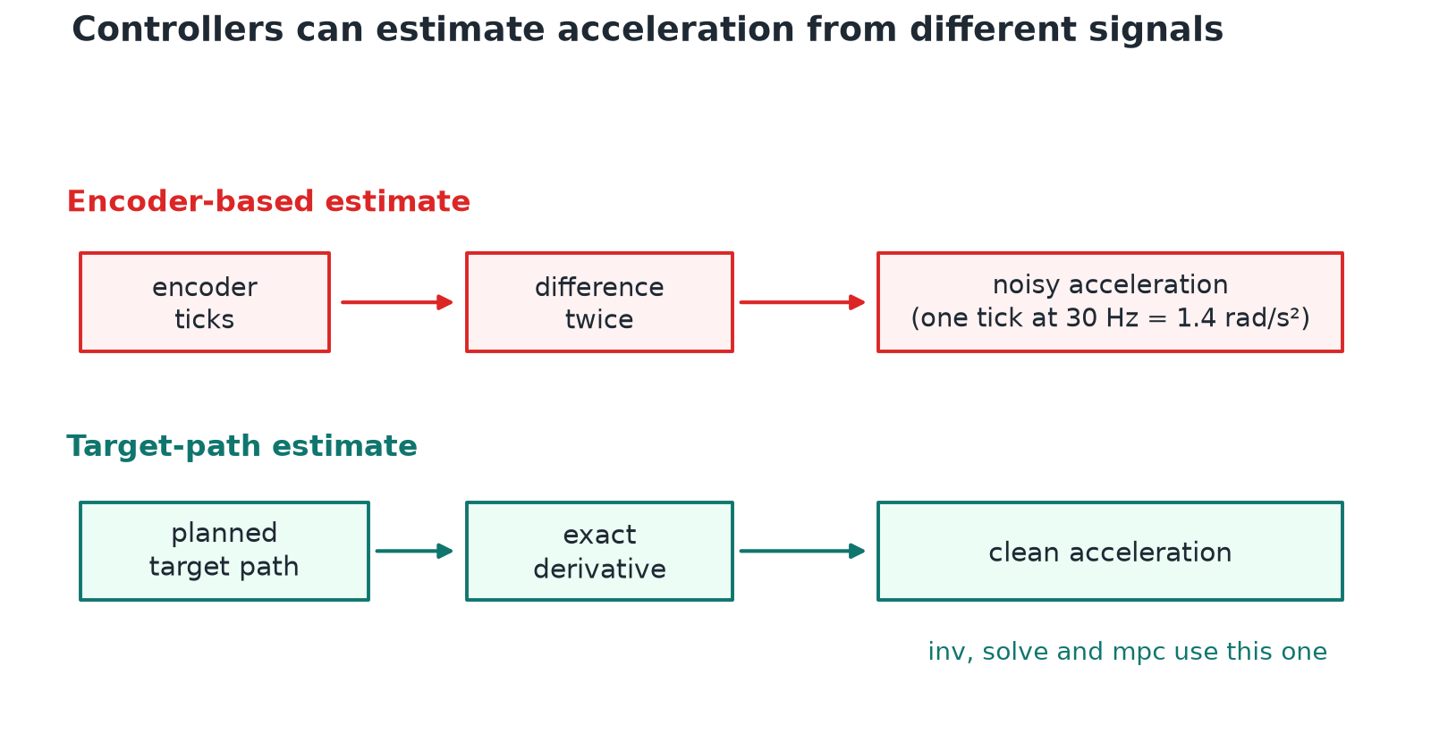
Two ways to get an acceleration. From the encoder: ticks, then two differences, then a noisy acceleration, 1.4 rad/s² per tick at 30 Hz. From the planned target path: an exact derivative and a clean acceleration, which inv, solve and mpc use. — My model-based controllers take the acceleration from the planned path, not from the encoder.

Partly. The model-based controllers avoid it, because inv, solve and mpc take the acceleration from the target path, which I know exactly and which has no sensor noise. One of my networks probably did run into it, though. It had 4 past readings as inputs, which in effect gave it a noisy acceleration estimate, and it did terribly in closed loop, as I describe in part 3. The study listed this as a likely cause, but I never tested it directly. Fitting a model from logs has the same problem, and the usual answer in the literature is to fit smooth periodic motions instead of differentiating raw readings (Swevers and colleagues, 1997).

A second amplifier: the one-step inverse

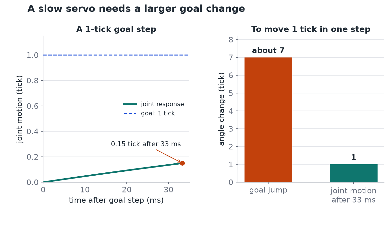
Left: after a goal step of one tick, the joint moves only 0.15 tick in 33 ms. Right: to move one tick in one step, the goal has to jump about 7 ticks. — One goal tick moves the joint about 0.15 tick in one step, so a one-step inverse multiplies errors by about 7.

There's another way to amplify noise, and this one shows up in almost all of my controllers. A one-step inverse asks which goal will put the joint on the target at the next step. The difficulty is that the servo responds slowly. In the simulator, moving the goal by one tick moves the joint by only 0.14 to 0.17 tick in one 33 ms step. The reason is that one goal tick only adds 13.64 × 0.001534 = 0.021 N·m of torque, and that torque first has to accelerate the arm against the damping, with a servo time constant of 78 ms, longer than two steps.

So to move the joint by one tick in one step, the inverse has to move the goal by about 1/0.15, roughly 7 ticks. Whatever the inverse sees gets multiplied by about 7, including the reading noise and any error in the model.

Predict first. Facts for this question. One goal tick is 1.534 mrad, so it adds 13.64 x 0.001534 = 0.021 N m of servo torque. That torque must first accelerate the arm, and the damping slows it: the servo time constant is d / kp = 1.058 / 13.64 = 78 ms, longer than one 33 ms step. In the MuJoCo copy, with the arm at 0.3 rad/s, a goal 1 tick higher puts the joint only 0.14 to 0.17 tick higher at the end of the step. The Fitted servo model chooses the goal that puts the joint on the next target at the end of ONE step. Now one reading jumps by +1 tick only because of rounding. The model then moves its next goal by about 5.6 ticks. Why so much? Answer: The one-step gain from goal to landing point is only about 0.14, so the solve multiplies any apparent error by about 1 / 0.14.

Estimate the angle instead of reading it

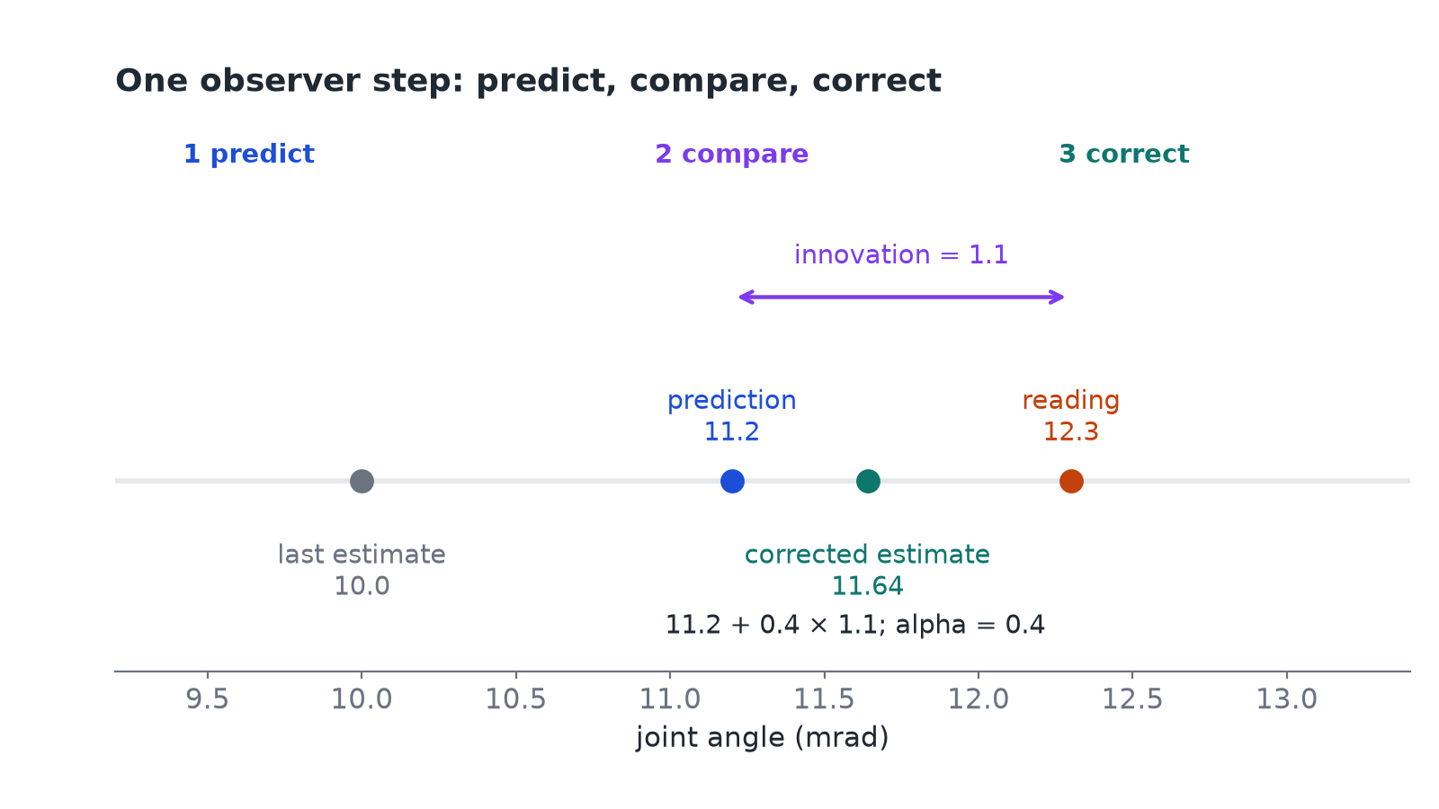
One observer step on a number line: the last estimate is 10.0, the model predicts 11.2, the reading is 12.3, the innovation is 1.1, and the corrected estimate is 11.2 plus 0.4 times 1.1, which is 11.64. — One observer step with α = 0.4: predict, compare with the reading, and move only part of the way.

This is the idea I found most fascinating in the whole project. Instead of trusting the reading alone, you use a model of the joint to predict where it is, and then you use the reading to correct that prediction, but only partly. The model knows the physics between two readings, and many readings together carry more information than a single one, so the estimate can end up finer than one tick.

The loop goes like this:

Predict: use the model to move the last estimate forward by one step.
Compare: subtract the prediction from the new reading. This difference is called the innovation.
Correct: move the estimate by a fraction α of the innovation.
Repeat at the next step.

This is called an observer. The simplest one is the alpha-beta filter, which estimates the position and the speed, and where you choose the fraction α by hand.

Does it actually help a controller? In the simulation study, the best model-based controller, Fitted, had an error of 0.398 mrad. With an alpha-beta observer feeding it (α = 0.4), the error went down to 0.268 mrad, and with a perfect sensor it would have been 0.228. The goal also stopped jittering: it changed by 39.1 mrad per step before the observer and by 5.9 after.

Predict first. The Fitted servo model fits 4 numbers of a simulated arm on 24 s of data. Its error is about 0.4 mrad, the same as the Exact model, which uses the true numbers. A fit on 1152 s of data is no better. The RMS of the rounding error of one reading is 1.534 / √12 = 0.443 mrad. Why can more data not lower the error? (A) 24 s is too short. A longer fit finds better numbers. (B) The model has the wrong form, so better numbers cannot help. (C) The fit is already nearly exact. Most of the 0.4 mrad comes from the tick rounding of the reading, which is about the same size, 0.443 mrad. (D) The simulated servo has a dead band that the model does not know. Answer: The fit is already nearly exact. Most of the 0.4 mrad comes from the tick rounding of the reading, which is about the same size, 0.443 mrad.

The Kalman filter

The obvious question is how to choose α, and that's where the Kalman filter comes in. The whole idea fits in one small calculation, and it's the one that made the filter stop looking like magic to me.

Two guesses are better than one

At each tick I have two guesses of the angle. The model predicts $q^-$ , and its error has a variance $P$ . The encoder reads $q_\text{read}$ , and its error has a variance $R$ . Neither is exact. So take a blend: start from the prediction and move a fraction $K$ of the way toward the reading.

\hat q = q^- + K\,(q_\text{read} - q^-) = (1-K)\,q^- + K\,q_\text{read}

The two errors are independent, so the variance of the blend is $(1-K)^2 P + K^2 R$ . It's a parabola in $K$ , and its lowest point is where the slope $-2(1-K)P + 2KR$ is zero:

K = \frac{P}{P+R}, \qquad \text{variance of the blend} = \frac{P\,R}{P+R}

That last fraction is the part I like. $\frac{PR}{P+R}$ is smaller than $P$ and smaller than $R$ , always. So the blend is better than the model alone and better than the sensor alone. That's how an estimate can get finer than one tick.

The two limits match intuition. If the prediction is bad ( $P \gg R$ ), $K$ goes to 1 and the filter believes the reading. If the reading is noisy ( $P \ll R$ ), $K$ goes to 0 and the filter believes the model.

Here is a number for my encoder. The rounding error is spread evenly over one tick, so $R = (1.534/\sqrt{12})^2 = 0.196\ \text{mrad}^2$ , an RMS of 0.443 mrad. Suppose the model is just as uncertain, $P = R$ . Then $K = 0.5$ , and the variance halves: the blend has an RMS of $0.443/\sqrt 2 = 0.31$ mrad, already below the rounding of a single reading.

The loop, with the gain in it

The Kalman filter is that blend, done at every tick, plus a rule for how $P$ changes. Between two ticks the prediction gets less certain, because the model isn't perfect: it adds a model noise $Q$ . After each reading it gets more certain, because the blend is better than either guess. For one joint and the angle alone, the four lines are:

\begin{aligned} \text{predict:}\quad & q^- = f(\hat q), && P^- = P + Q\\ \text{gain:}\quad & K = \frac{P^-}{P^- + R}\\ \text{correct:}\quad & \hat q = q^- + K\,(q_\text{read} - q^-), && P = (1-K)\,P^- \end{aligned}

$f$ is the model step, and $q_\text{read} - q^-$ is the innovation from the observer section. Compare it with the alpha-beta filter: the correct line is the same, with $K$ in place of α. The only new part is that $K$ comes from $P$ , $Q$ and $R$ instead of from my hand.

When $Q$ and $R$ stay constant, $P$ and $K$ settle to fixed values after a few ticks. At that point the Kalman filter is an alpha-beta filter with the right α. So the way I think about it now is that the alpha-beta filter is a Kalman filter where you picked the gain by hand and froze it.

The same loop with more than one number

A real filter keeps several numbers per joint, for example the angle $q$ and the speed $w$ , in a state vector $x$ . $P$ becomes a table (a matrix) of the uncertainty of each number and of how their errors move together. The model step is a matrix $F$ , and the encoder only reads the angle, which a row $H = [1\ 0]$ picks out:

x^- = F x, \quad P^- = F P F^\top + Q, \quad K = \frac{P^- H^\top}{H P^- H^\top + R}, \quad x = x^- + K\,(q_\text{read} - H x^-), \quad P = (I - K H)\,P^-

$K$ now has one row for each number in the state. The encoder never measures the speed, but the filter still corrects it, because the speed error and the angle error are linked through $F$ : a wrong speed today makes a wrong angle tomorrow. The "extended" Kalman filter does the same with a model that isn't linear, and computes $F$ again at each tick as the slope of the model.

Two things you can observe

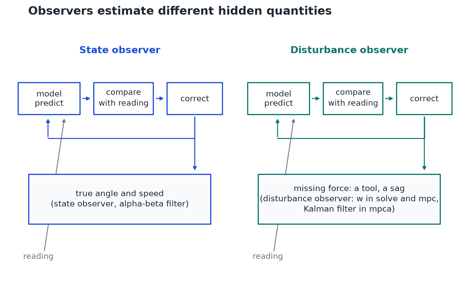
Two observers with the same predict, compare and correct loop. The state observer estimates the true angle and speed, like the alpha-beta filter. The disturbance observer estimates a missing force, like ŵ in solve and mpc or the Kalman filter in mpca. — The same loop can estimate the state of the joint or the force the model is missing.

The same idea can estimate two quite different things, which confused me for a while. A state observer estimates the true position and speed, and the alpha-beta filter above is one. A disturbance observer estimates what the model is missing, like a tool in the gripper or a sag the model didn't expect. It works by adding the missing torque $d$ to the state, as one more number that the model expects to stay constant:

J\,\dot w = \tau_\text{servo} - (\text{the forces the model knows}) + d, \qquad d_{k+1} = d_k + \text{a small random step}

The encoder never sees $d$ . The filter can still learn it, for the same reason as the speed: $d$ changes the speed, and the speed changes the angle. So when the joint lands lower than the prediction at tick after tick, the innovation keeps the same sign, and $d$ moves a little in the same direction at each tick until the prediction matches the readings again. The gain of $d$ is the slope of that link, how much $d$ is probably wrong when the angle is wrong by one radian. Nothing in the filter knows the cause: $d$ takes any steady torque the model misses.

My solve and mpc controllers already keep a simple disturbance observer called $\hat w$ . At each step the model predicts the next reading, the prediction error tells the controller that something is missing, and $\hat w$ moves a small part of the way toward explaining it, dt / 0.3 s of the way each step. mpca replaces that with a Kalman filter that has a fast part for a load and a slow part for sag. I go through both in part 3.

Where I was wrong: is mpca the observer?

When I first learned about observers, I thought that was exactly what mpca adds. It's the same family, but it estimates something else. mpca's Kalman filter is a disturbance observer that estimates the missing force, while the alpha-beta filter is a state observer that estimates the true angle.

Where I was wrong: is ŵ a Kalman parameter?

I thought $\hat w$ was a setting. It's actually an estimate that changes during the run. For each joint, it's the steady part of the error that the model doesn't explain, in goal units, and the controller subtracts it from the goal.

A prediction I got right: would mpc chatter less with an observer?

Yes. The observer's position is smoother than the reading, so the goal flips between two ticks less often, which removes one cause of chatter. The reversal gate in part 3 handles another cause, which is plans that keep crossing the dead band back and forth.

What's next

With a model, a controller can see the joint more finely than one tick. Part 3 puts the whole equation to work: it writes one general formula for the goal, and shows where the observers of this part plug into it. Part 4 shows that a network can do the job of the disturbance observer, with more freedom.

← All writing