I've been trying to find out whether a robot controller can be more accurate than the classical ones. To answer that, I first had to understand how the classical controllers work and which problems each of them fixes, and then test them on my own SO-101 arm and in the Genesis simulator. This series is what I learned along the way.
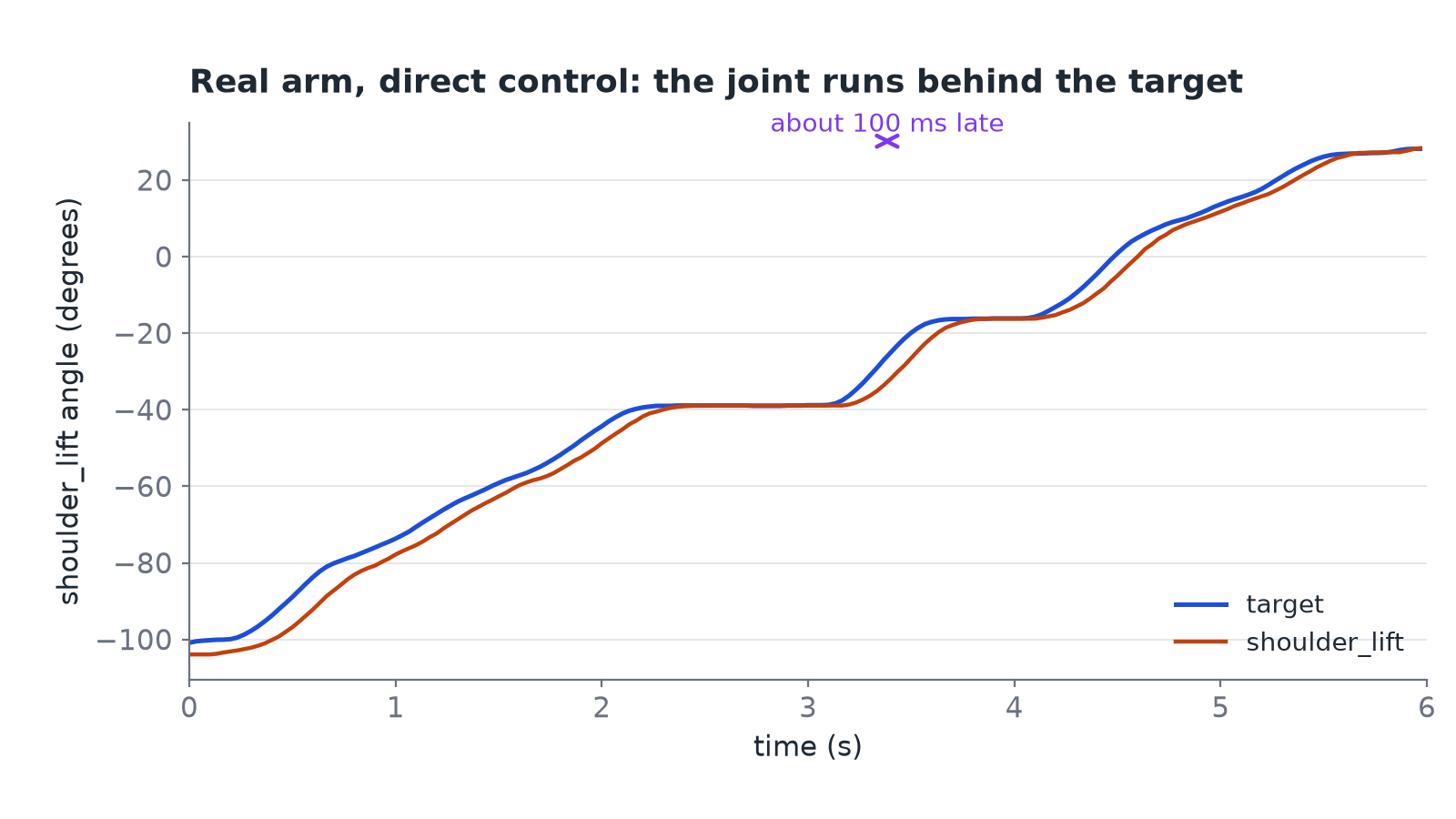
When I send my arm a smooth path to follow, it doesn't quite follow it. It arrives a little late, it stops a little short, and when it's supposed to hold still it sags slightly below the angle I asked for. With the default LeRobot setup running at 30 Hz, the joints end up 22.5 mrad away from the path on average, which is about 1.3 degrees. That doesn't sound like a lot until you remember the gripper sits 30 cm out at the end of the arm, and that I'd like it to pick up something as small as a screw.
I call the default controller direct: at each step, it sends the target angle to the servo, unchanged. This is what LeRobot does.
So I wanted to understand why the arm misses. This article writes one joint of the arm as a single equation, starting from the physics everyone knows, torque equals inertia times acceleration. Then it goes through the equation one term at a time. Each term is one way the arm can miss, and for each one I give an example and the size of the error on my arm. Part 2 is about the sensor, and part 3 groups the controllers by the term of this equation that they fix.
Target, goal, gap
Three words confused me for a long time, mostly because I used them as if they meant the same thing. In this series each one has a single meaning:
- the target is where I want the joint to be, either from a policy or from a path I planned;
- the goal is the number I actually send to the servo;
- the gap is the difference between the goal and where the joint really is.
Why would I ever send a goal that isn't the target? The easiest way I found to think about it is to picture the servo as a spring. The goal is where you attach one end of the spring and the joint hangs on the other end. Gravity pulls the joint down, and the spring stretches until it pulls back just as hard. The important part is that the spring only pulls when it's stretched, so the servo can only make torque when there's a gap.
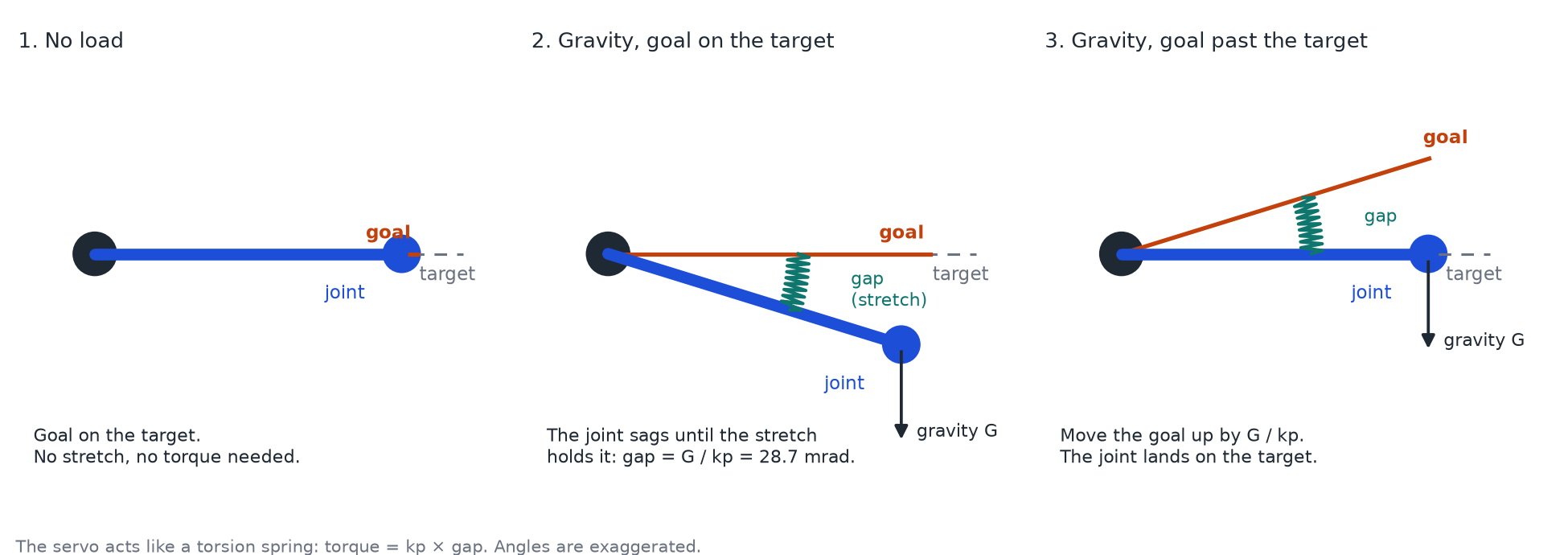
As far as I can tell the picture is accurate for the main part of the servo. Its P term follows a spring law: the torque is times the gap, the same way a torsion spring pushes back harder the more you twist it. The real servo adds a few things on top of that spring, like damping, a small dead band where it makes no torque, and a maximum torque, and I come back to each of them later.
That means if I put the goal exactly on the target, the joint can't actually stay on the target. It has to sag until the stretch is large enough to hold the arm up, and the size of that sag is the gravity torque divided by the stiffness of the spring:
The units are N·m ÷ (N·m/rad) = rad, so a torque divided by a stiffness gives you an angle. On the simulated shoulder at the example hold pose, gravity is 0.391 N·m and the servo stiffness is 13.64 N·m/rad, which gives a sag of 28.7 mrad.
The same reasoning works for every other force on the joint: friction, a tool in the gripper, the force needed to speed the joint up, the damping that resists motion. Each of them needs a bit more gap, and if the goal stays on the target, all of that extra gap shows up as error.
So the problem I kept coming back to was really just this one: where should I put the goal? Every controller in the series is a different answer to that question.
Units: ticks, mrad and degrees
The encoder counts 4096 ticks per turn. One turn is 2π rad, so 1 tick is 1.534 mrad, or 0.088°. One degree is 17.45 mrad, which is about 11.4 ticks. I use mrad in this series because most of the errors are somewhere between a few mrad and a few tens of mrad.
Glossary
- Target (): where I want the joint to be.
- Goal: the number I send to the servo.
- Reading (): the angle the encoder reports, in whole ticks.
- Tick: one encoder step, 1.534 mrad.
- Gap: the goal minus the joint angle. The servo makes torque only from the gap.
- Stiffness (): torque per radian of gap, in N·m/rad.
- Damping (): torque per rad/s of speed that resists motion. is the lag it causes.
- Dead time (): the pause between a new goal and the first motion of the joint.
- Goal hold: the goal stays the same for a whole control step.
- Dead band: a small gap where the servo makes no torque.
- Wet (viscous) friction: friction that grows with speed. Dry (Coulomb) friction: friction of a fixed size that opposes motion.
- Sag: the steady error under gravity, when the goal is on the target.
- Feedforward: moving the goal ahead using what I know in advance, like the path and the physics.
- Feedback: correcting the goal from the error I measure.
- Inner loop: the servo's own loop. Outer loop: my controller on the computer, which only sends goals.
One equation for the joint
Physics gives a simple recipe for the goal. For a joint that turns, Newton's second law says : the torque equals the inertia times the angular acceleration. I know the target path in advance, so I can take its second derivative and compute the torque the joint needs. The servo gives times the gap, so the goal that gives exactly that torque is
If my arm obeyed only , that one line would be the whole series. It doesn't, because each side of the equation hides more terms. This is the equation of one joint in the form I use for the rest of the series:
Each term has one meaning:
- Servo torque, : the servo pushes in proportion to the gap. The goal it uses is seconds old (the dead time), and it measures the gap from the reading , which is rounded to whole ticks. The formula doesn't show two more limits: a dead band where the servo makes no torque, and a maximum torque.
- Mass, : the torque to speed the joint up or slow it down. changes with the pose and with a payload.
- Gravity, : the weight of the links beyond the joint. It changes with the pose.
- Wet friction, : friction that grows with speed.
- Dry friction, : friction of a fixed size that always opposes the motion.
- Speed coupling, : the torque that the speed of one joint puts on another joint, the Coriolis and centrifugal effects.
I wrote the force terms from the largest to the smallest on my arm. With every term known exactly, the same step as before gives the ideal goal: read the target one dead time ahead, and add every torque divided by :
The derivatives come from the target path, which I know exactly, not from the readings. Every term I leave out or get wrong comes back as error. The figure shows the problems that come out of each term and their size on my arm. Select a term to keep only its problems; the names link to their sections.
Two kinds of problem in the figure aren't forces at all. The dead band, the torque limit and the dead time change the servo torque itself: they decide how much torque a goal gives, and when. The ticks change what the controller reads, so they also spoil every speed or acceleration computed from the readings. That's why I kept them on the left side of the equation.
The rest of this article goes through the equation from left to right: the servo, the mass, and then the forces. At the end, one measured step puts all the terms together.
The servo side
The servo sits in the middle
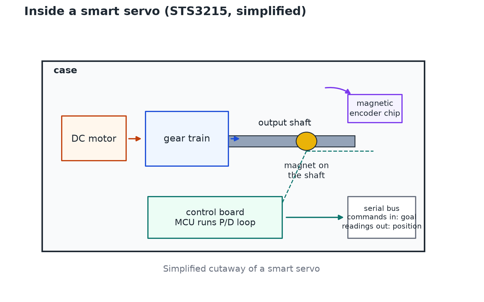
Something that took me a while to accept is that I can't actually drive the motors of my arm. I can only talk to the servos. Each joint of the SO-101 is a smart servo, the STS3215, with a motor, a gearbox, an encoder and a small controller inside. That little controller runs its own loop: it reads the encoder, compares it with the goal I sent, and decides how much power to give the motor. I never get to set the motor power myself. All I can do is send goals.
So there are really two loops stacked on top of each other. The inner loop runs fast inside the servo and drives the motor. The outer loop runs on my computer at 30 or 60 Hz, reads the joint angles and sends new goals.
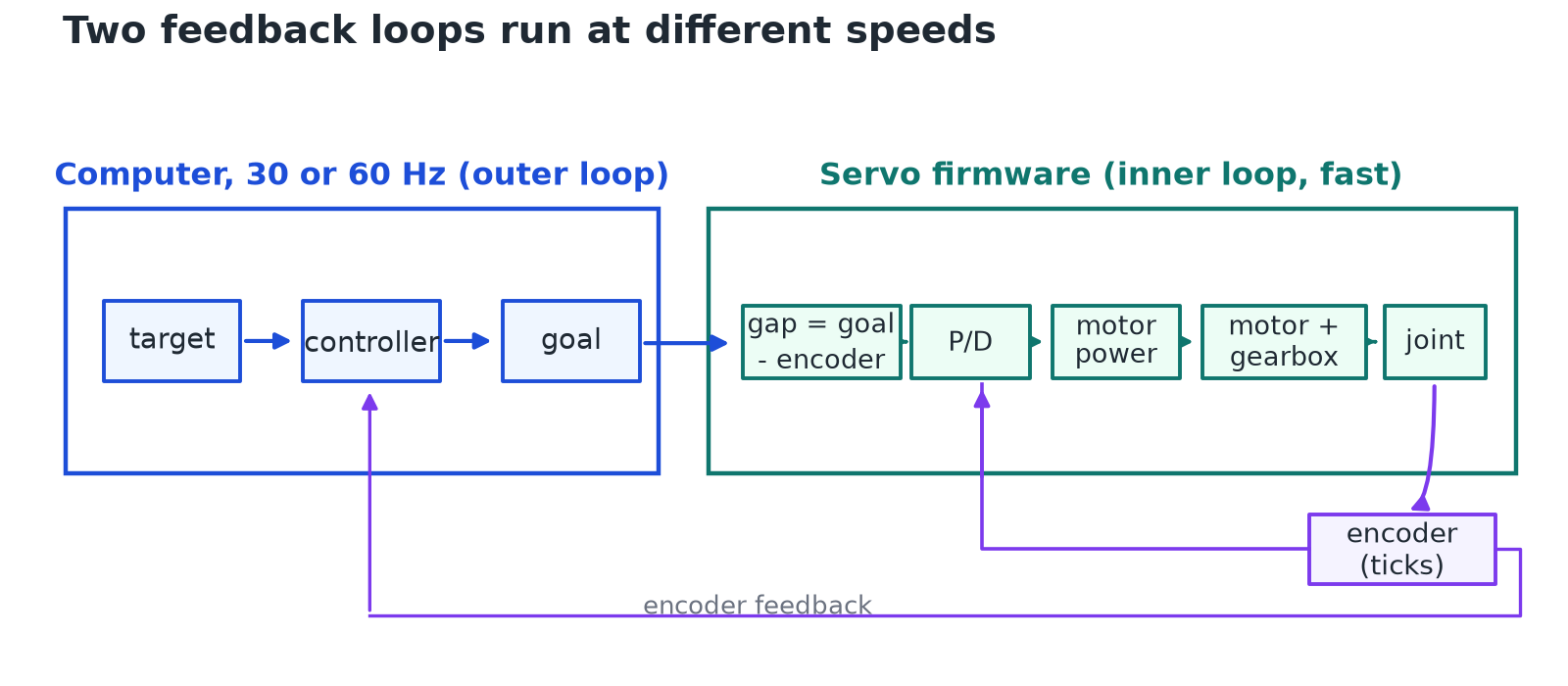
Every controller in this series lives in that outer loop. None of them changes how the servo works inside; they can only try to send it a better goal.
What PID actually means
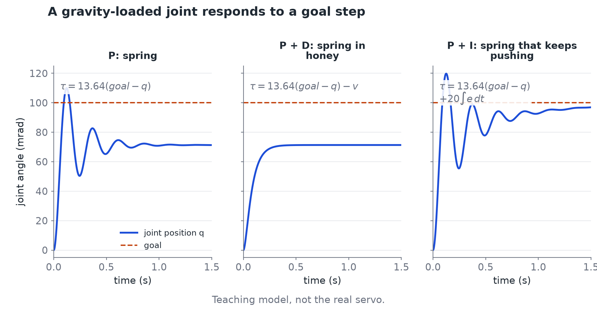
I'd seen "PID" many times before this project without really knowing what it did. On a servo, each of the three letters turns out to be something you can picture physically. P, the proportional term, pushes in proportion to the gap, so it's the spring from earlier, and its gain is a stiffness in N·m/rad. I, the integral term, adds up the error over time, so if a small error refuses to go away, the integral keeps growing until it pushes hard enough to remove it. D, the derivative term, pushes against the speed, which acts like damping, a bit like moving the joint through honey.
Where I was wrong: is kp the inertia?
At first I thought was some kind of inertia. It isn't. Inertia (kg·m²) resists changes of speed and doesn't care where the goal is, while is a stiffness: how much torque you get per radian of gap. On this servo it depends on the firmware P register, the supply voltage, the motor and the gearbox.
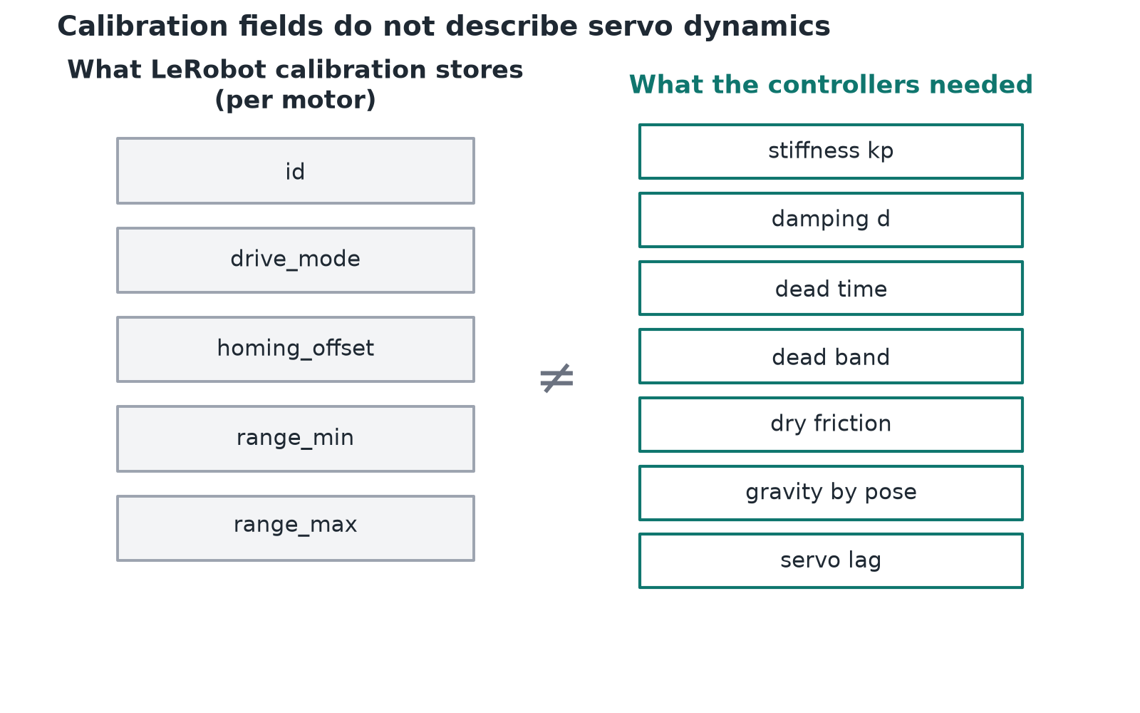
Knowing that, I was curious what LeRobot actually sets up when you calibrate the arm. I expected some measurement of each joint, but my calibration file stores five integers per motor: the motor id, the turn direction, a homing offset, and a minimum and maximum position. My shoulder_lift, for example, has a homing offset of 941 and a range from 844 to 3214 ticks. Then, every time the arm connects, LeRobot writes the same default servo settings to every motor: position mode with P = 16, I = 0 and D = 32, plus a 50 % torque cap on the gripper, which the code comments say is there "to avoid burnout".
So the control loop is identical on every SO-101, and nothing in it knows the stiffness, damping, friction, delay or gravity of my particular arm. I'd describe LeRobot's calibration as geometric, because it finds where zero is and where the limits are. It isn't a dynamic calibration, which would tell you how this specific joint responds to a goal, and that second kind is what the rest of this series is about.
I also wondered why the integral is set to zero. As far as I can tell it isn't documented, so this is a guess, but I think the gripper is a likely reason. When the gripper closes on an object it never reaches its goal, and an integral term would keep growing until the motor is pushing at full torque and heating up. The price of I = 0 is the steady sag from earlier, and the feedback controllers in part 3 add an integral back, outside the servo.
Dead time
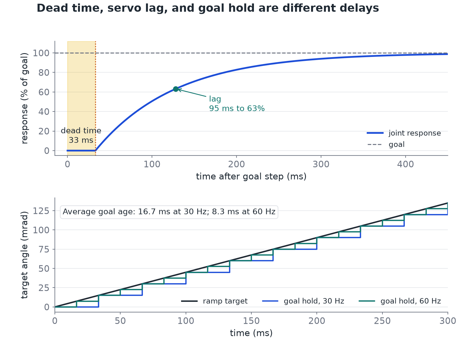
When I first said "the arm is late", I was mixing up three different things, and they don't have the same fix. Two of them are on the servo side: the dead time and the goal hold. The third, the lag, comes from wet friction, and I come back to it with the forces.
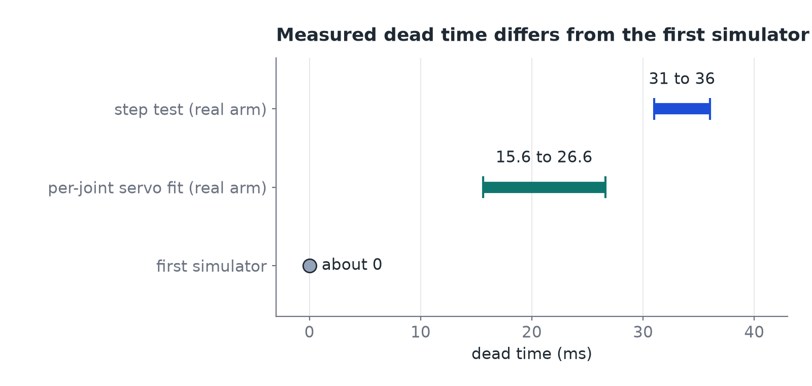
When I send a new goal, nothing happens for a short while, and only then does the joint start to move. That pause is the dead time, the in . On my real arm a step test measured 31 to 36 ms, and a per-joint fit of the servo model gives 15.6 to 26.6 ms. The two methods don't measure quite the same thing: the step test looks for the first visible motion after a jump of the goal, while the fit picks the delay that best explains whole recorded motions together with a lag and a dead band. I haven't fully resolved the difference between them. The simulator I started with had almost no dead time at all, which made it one of the biggest differences between the simulator and the real arm.
Dead time is hard to deal with because feedback can't fix it. Any correction I send arrives at least one dead time late, so if I push hard on information that's already old, I overshoot. The only real fix is to predict, and send the goal for where the target will be one dead time from now, which is the in the ideal goal. It also doesn't go away with a faster loop. 33 ms happens to be close to one step at 30 Hz, but at 60 or 100 Hz the dead time is still there.
In this widget, inv is a controller that sends the target one dead time ahead; part 3 explains it.
Goal hold
My controller sends a new goal once per step, every 33.3 ms at 30 Hz. Between two steps the goal stays still while the target keeps moving, so on average the goal I'm following is half a step old, about 16.7 ms. This one does shrink with a faster loop.
Am I limited to 33 ms?
No. 33 ms is the LeRobot loop rate (30 fps), which was picked for the cameras and the policy. The servo runs its own loop much faster inside. The practical limits are the serial bus, the latency of the USB adapter, and the Python overhead. I haven't measured those yet.
Dead band
The servo firmware has a small band of gap where it makes no torque at all, so the motor doesn't buzz while it holds still. On my arm it's between 8.1 and 21.0 mrad, depending on the joint, which is 5 to 14 ticks. Inside the band, moving the goal does nothing. Outside it, the servo pushes as if the gap were smaller by the width of the band.
This term breaks the "divide by " recipe. To push up, the goal has to sit above the band; to push down, below it. So the right goal jumps by twice the band each time the motion reverses, and there is no smooth formula for it. The simulator I started with had no dead band.
Torque limit
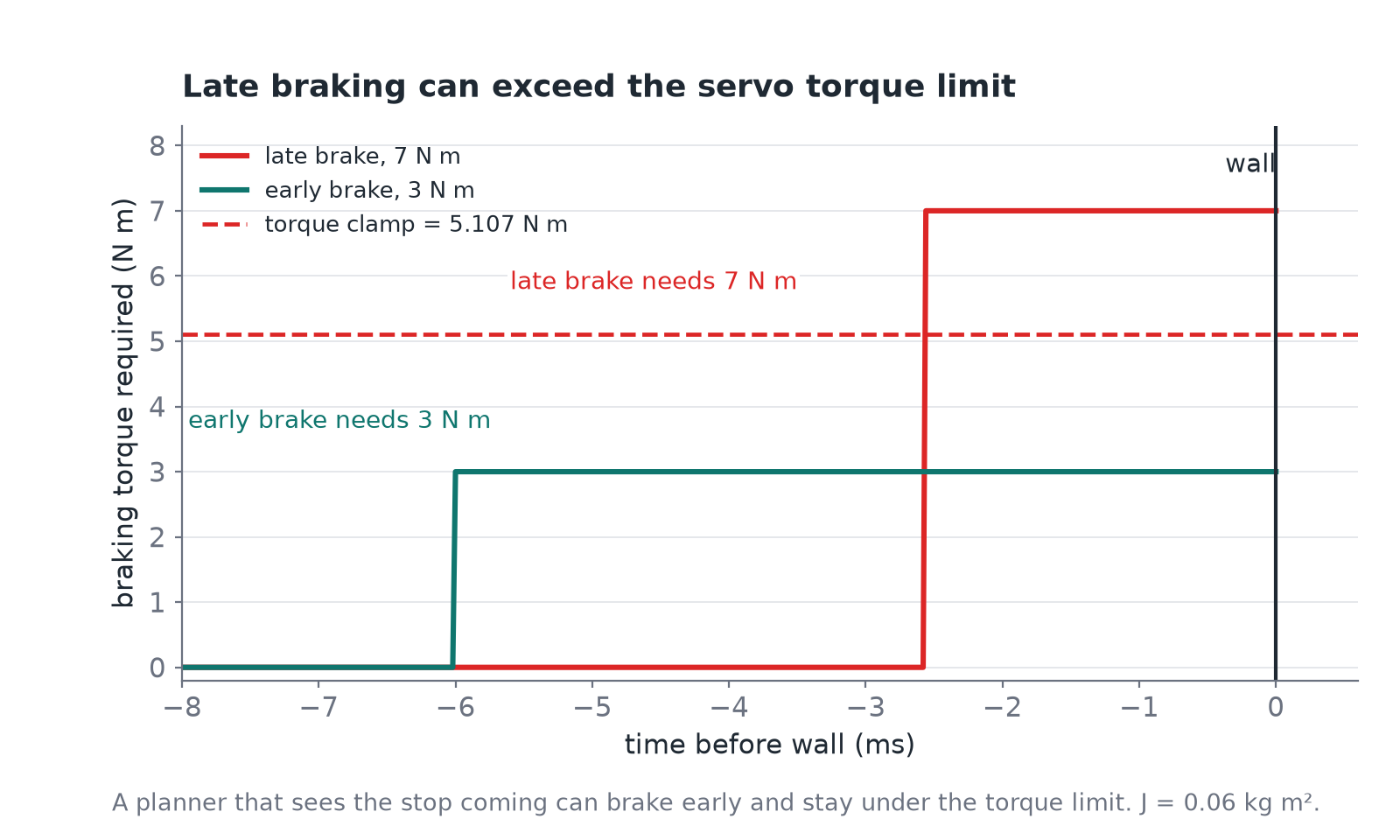
The servo also has a maximum torque, about 5.1 N·m in the simulator. If a motion asks for more than that, there's no goal that can deliver it, and the only way out is to start braking or accelerating earlier. Part 3 shows how a planner can do that.
Heat
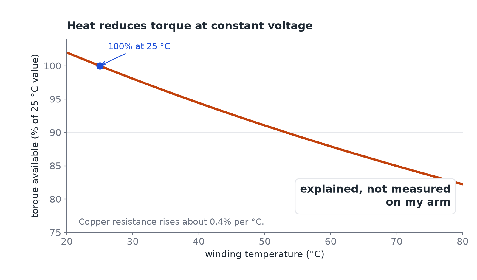
A hot servo is weaker, so itself drops. The resistance of the copper rises by about 0.4 % per °C, so at the same voltage the current and the torque both drop, and the magnets also weaken a little when they get hot. The STS3215 has an over-temperature cut-off. I haven't measured any of this on my arm, and the simulator has no temperature model, so for now heat is on the list of effects I can describe but not yet correct.
The mass term: inertia and a payload
The first term on the right is , the torque to speed the joint up or slow it down. isn't one number: it's the inertia the joint sees, and it changes with the pose, because an arm stretched out is harder to turn than a folded one. At the speeds I record, this term is small on my arm: 2.1 mrad in the example step at the end of this article.
A payload changes , and it also adds weight, so it changes too.
When the arm picks up a tool, it needs more torque to hold it against gravity. In the simulator, a 150 g tool at the home pose adds about 0.38 N·m on the shoulder lift joint, and a 200 g tool adds about 0.50 N·m. On a hold, the weight is the part that matters. In a fast motion, the extra mass also has to be accelerated and stopped, and part 3 has a test of that.
Where I was wrong: does the tool weight flip sign?
I thought the tool's weight flipped sign when the arm reversed. It doesn't, because gravity always pulls down. Friction flips with the direction of motion, gravity doesn't. What changes with the pose is the lever arm, so the tool torque depends on where the arm is.
The force terms
Gravity changes with the pose
The gravity torque on a joint depends on how far the links beyond it stick out horizontally. With the arm stretched out flat, the shoulder carries the largest torque, and with the arm pointing straight up it carries none.
The clip also shows an error I can't explain yet. Only the shoulder moves in this test, and the elbow target stays still. But the elbow stays about 70 mrad (4°) away from its target in both poses. If gravity caused it, the error would change between the tucked and the reaching pose, and it doesn't. I see the same 70 mrad in every recording where I moved one joint at a time. My guess is a fixed offset in the elbow calibration, but I haven't checked it.
The servo models I fitted capture this through the angle of each link from vertical, which is the shoulder angle, then shoulder plus elbow, then shoulder plus elbow plus wrist. The sines and cosines of those angles have the same shape as the gravity torque of a chain of links.
Wet friction becomes a lag
Friction ended up being one of the most interesting parts of this project for me, mostly because it isn't one thing. It's easier to understand by adding the pieces one at a time, and the equation has two of them.
The first piece is viscous friction, which I kept calling wet friction, the term. It grows with speed, and in a servo a lot of it comes from the motor itself: a spinning motor produces a back voltage, the back-EMF, that resists the motion. In the simulator it's folded into one damping constant, 1.058 N·m·s/rad.
What surprised me is that this force turns into time. Damping needs a torque when the joint moves at speed , so the servo needs a gap of to provide it. But if you look at that gap from the target's point of view, it's exactly the distance the target travels in seconds. In other words, damping makes the joint behave as if it were running a fixed time behind the target:
The units work out as (N·m·s/rad) ÷ (N·m/rad) = s. The picture I use is pulling a box through honey with a spring: your hand always has to stay a fixed stretch ahead of the box. Pulling harder makes the box go faster, but your hand is still ahead of it. More torque doesn't remove the lag. What removes it is putting the goal ahead of the target by that amount, which is what control people call feedforward.
The last conversion closes the loop. If the joint runs behind and moves at speed , the error is , and the units are s × rad/s = rad again. So three units, N·m of torque, mrad of error and ms of lag, can often be turned into one another.
The measured lag on the simulated robot was 105.5 to 108.4 ms, so the simple estimate is about 12 % low, but it gets the size right. On the real arm the servo fit gives 87 to 105 ms.
Where I was wrong: 77 ms
My answer was 77 ms. I'd forgotten that the goal only changes once every 33 ms step, so on average the goal I'm following is already half a step old, which adds another 16.7 ms.
Dry friction makes a band
The second piece is Coulomb friction, or dry friction, the term. It has a fixed size, 0.196 N·m in the simulator, and it doesn't depend on speed. It just opposes the motion.
Where I was wrong: does dry friction become wet friction?
I thought dry friction turned into wet friction as the joint sped up. It doesn't. They're two separate terms that add together. In one test the dry friction seemed to disappear, but that was only because the joint crept, so the spring ended up carrying more of the load and friction had less to carry.
The part I found most surprising is what dry friction does to a joint at rest. Write the torques on a joint that holds still under gravity. The servo pushes up with , gravity pulls down with , and friction adds a torque of its own:
At rest, dry friction isn't a fixed number. It takes any value between and that keeps the joint still. So the servo doesn't need one exact gap. Any gap works if friction can make up the rest:
With the simulator numbers, = 0.391 N·m, = 0.196 N·m and = 13.64 N·m/rad, that's any gap from 14.3 to 43.0 mrad. Without friction there would be one answer, = 28.7 mrad, in the middle of the band.
Where in the band does the joint stop? Friction always pushes against the motion, so it depends on where the joint comes from:
- The joint falls into place (gravity wins, the joint moves down): friction pushes up and helps the servo. The joint stops as soon as , at the low edge.
- The joint is pushed up into place (the servo wins, the joint moves up): friction pushes down, against the servo. The joint stops at , at the high edge.
The clip below tests the first case. The arm holds still, on its target, and a 200 g load grows slowly in the gripper, like sand that fills a cup. The load pulls shoulder_lift with = 0.614 N·m. Without friction, the joint should sag by = 45 mrad. With friction, it should stop at = 31 mrad, because friction carries of the load. I ran the same test three times, with three friction models.
| Friction model | shoulder_lift error at 4 s | at 12 s |
|---|---|---|
| None | 44.8 mrad | 44.8 mrad |
| Hard: stick or slip | 31.3 mrad | 31.3 mrad |
| Simulator: soft | 33.9 mrad | 43.4 mrad |
Without friction, the arm sags the full 45 mrad. With hard friction, it stops at 31 mrad, the low edge of the band, and stays there: friction carries 0.196 N·m of the load for as long as the arm holds still. With the simulator's own friction, the arm first stops near 31 mrad too, and then it slowly creeps down, 38 mrad at 6 s and 43 mrad at 12 s, toward the frictionless 45 mrad. The creep isn't physics. A joint at rest has no reason to start moving again.
Why the simulator creeps
The creep comes from how the simulator solves friction. Exact dry friction is awkward for a solver. When the joint is stuck, the friction force isn't given by a formula, only by a limit: any value between and . The solver has to decide, at every step and for every joint and contact, which ones stick and which ones slip. That is a switching problem with no smooth solution, and it gets slow and fragile with many contacts.
MuJoCo, which made this clip, avoids the switching. It makes friction a soft constraint: instead of forcing the speed of a stuck joint to be exactly zero, it lets friction grow very steeply with a tiny speed, like a very stiff damper (its time constant here is solref = 0.02 s). Each step then becomes a smooth optimization with one answer, which is fast and stable. The price is that a joint that friction holds against a load always slides a little, so it creeps. Genesis uses the same kind of soft constraint, which is where my first creep numbers came from.
The hard version in the middle panel is mine, and writing it showed me why simulators avoid it. At each step, the rule checks every joint: if it's stopped and friction can hold it with at most , it stays stuck; if not, it slides with friction against its motion. My first version almost never saw a speed of exactly zero, because in discrete steps the speed jumps across zero. So friction flipped sign every step and pushed the arm past the band edge to 37 mrad. It needed one more rule, "a speed that changes sign counts as stopped", before it stopped at 31 mrad. A real geared servo usually sticks like the middle panel. I haven't measured that on my arm.
For control, the band means the same target can give two different errors, depending on the direction the joint came from. A fixed goal offset can't fix both.
The same friction helps on a hold and hurts in motion
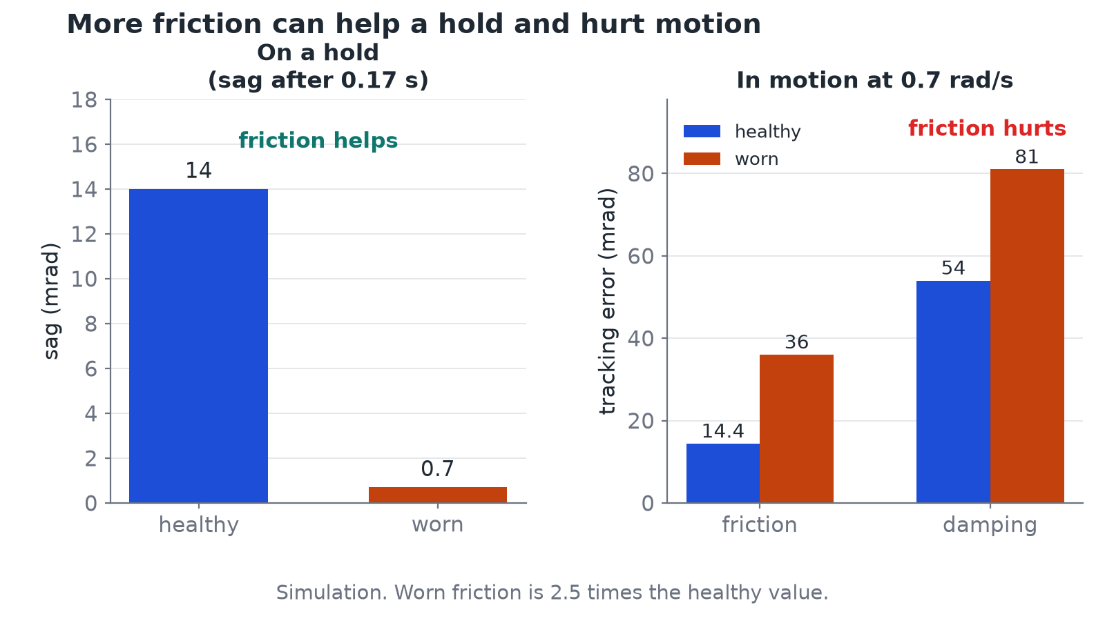
To see how the different terms interact, I like to look at a worn robot, with friction multiplied by 2.5, so = 0.49 N·m. That's more than the gravity torque at the example hold, 0.391 N·m. On a hold, friction helps: it carries the whole load at first, and the joint sags only 0.7 mrad after 0.17 s, against 14.0 mrad on the healthy robot, before the soft friction slowly creeps to 17.2 mrad at 6 s. In motion it's the opposite. Friction adds 36 mrad of lag, against 14.4 mrad on the healthy robot, and the extra damping at 0.7 rad/s adds 81 mrad, against 54 mrad.
Since most of the score comes from paths that move, the worn robot ends up much worse overall: 64.8 mrad on a multisine path (a sum of sine waves) and 73.4 mrad on a path shaped like the output of a robot policy.
Low speed is the hard case
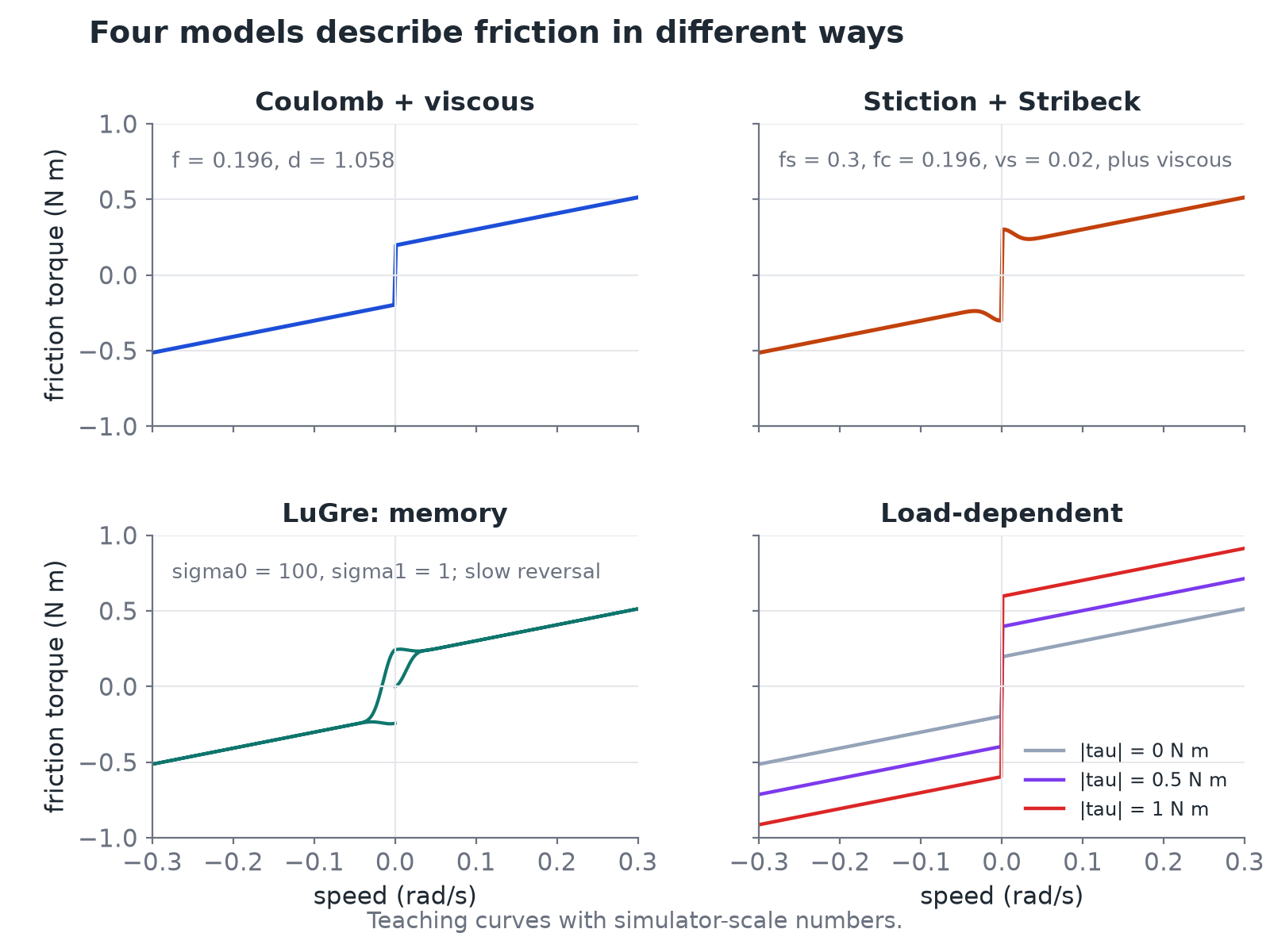
Real friction has more pieces than the two terms of my equation, and most of them show up at low speed:
- stiction and breakaway: at rest, the joint needs more torque to start than to keep moving;
- the Stribeck effect: right after breakaway, friction drops as the speed rises, before viscous friction takes over, and that dip is what makes low speed unstable, with the joint sticking, jumping and sticking again;
- LuGre friction: friction has a memory, with a tiny "pre-sliding" motion before a real slide;
- load-dependent friction: friction grows with the torque the servo is pushing, .
To find out which of these mattered on my arm, I fitted a Genesis model of the arm to real logs and compared friction models one at a time on real motions the fit hadn't seen (replayed in simulation):
| Friction model | shoulder_lift error (mrad) |
|---|---|
| Coulomb only | 21.8 |
| Load-dependent | 18.9 to 19.2 |
| Load-dependent + LuGre | 15.9 to 16.2 |
| Fitted servo model, for reference | 15.9 |
Stribeck gave no gain, and LuGre alone gave 3 % to 8 %. These runs didn't use exactly the same settings, so I'd treat the ranking as a first pass rather than a final answer.
Friction also decides where a stuck joint stops: at the first point where the drive torque falls below static friction. So the hold position can scatter by up to , which is 12.4 mrad on shoulder_lift. And compensating friction has its own risk, because a controller that overcompensates at low speed can make the loop unstable (Canudas de Wit and colleagues, 1991). That's why the controllers in part 3 smooth the friction term near zero speed and refuse small reversals across the dead band.
Speed coupling
This one is even weirder: the speed of one joint creates a torque on another joint. The picture I have in mind is a trebuchet. When the arm swings fast, the sling flies outward. On the SO-101, when the base pan spins quickly, the elbow has to hold the forearm in, which is the centrifugal part. When two joints move at the same time, each one also feels a torque that depends on the product of the two speeds, which is the Coriolis part. Both are in the term.
The widget shows a teaching model: two links seen from above, with SO-101-sized lengths and masses, and no gravity. The arrows are the two forces that the forearm feels when you watch it from the turning upper arm. The centrifugal force pushes the forearm out from the shoulder, and it grows with the square of the shoulder speed. The Coriolis force pushes sideways, and it appears only when the elbow moves while the shoulder turns. Each force puts a torque on a joint that no single-joint model expects.
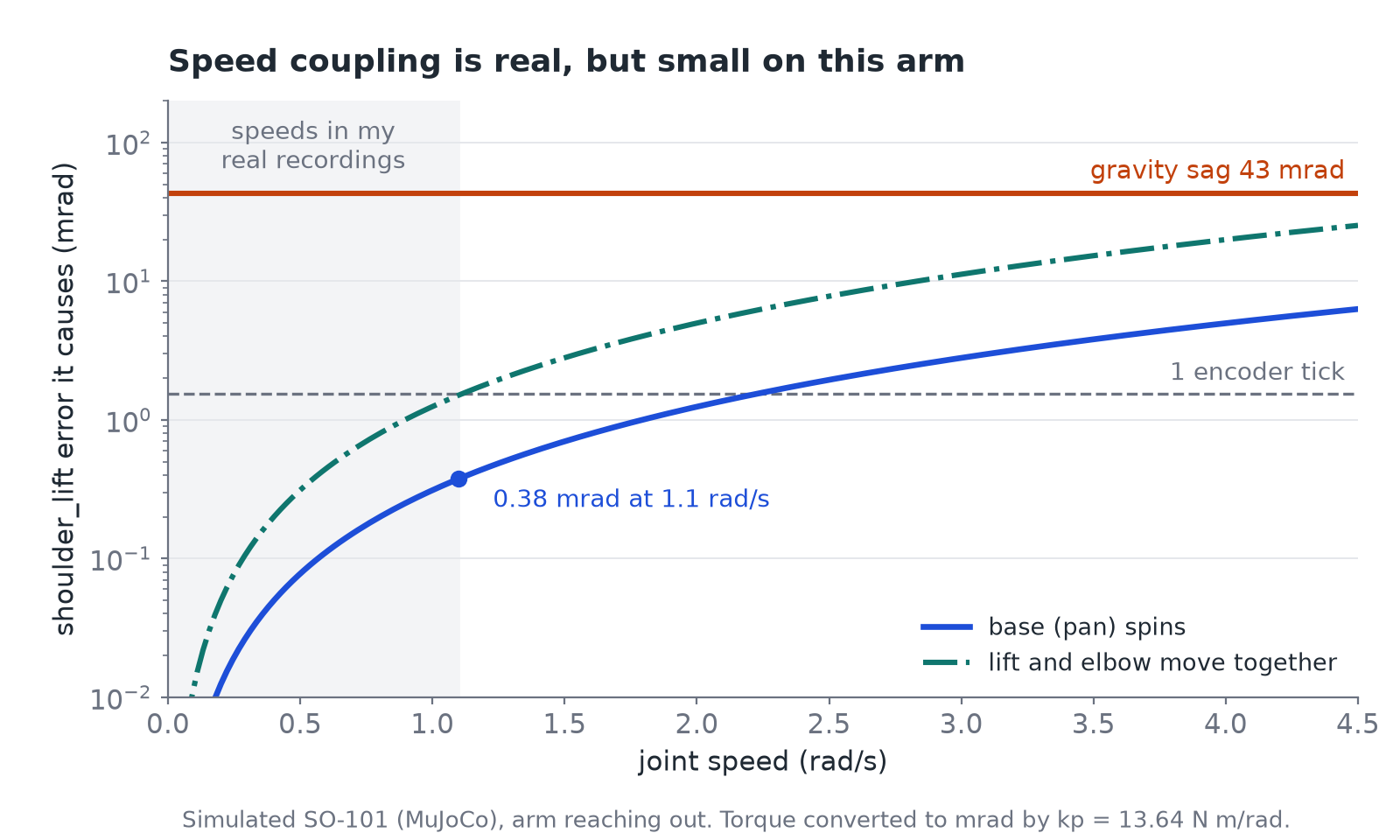
On this arm, the effect is small. With the arm reaching out, a base that spins at 1.1 rad/s (about the fastest speed in my real recordings) pushes shoulder_lift by 0.38 mrad, a quarter of one encoder tick. Lift and elbow moving together at that speed cost 1.5 mrad, about one tick. Gravity at the same pose costs 43 mrad. The coupling grows with the square of the speed, so it matters for a fast or heavy arm, but on a slow $100 arm it is near the bottom of the list.
The same effect, measured on the full simulated arm
The sensor side
Every term above uses the true angle , but the controller only ever sees the reading , in whole ticks of 1.534 mrad. Rounding alone leaves an error of 0.443 mrad RMS, and it gets much worse when a controller takes differences of readings to get a speed or an acceleration: at 30 Hz, one tick of error becomes 1.4 rad/s² of acceleration error. That's why the ideal goal above takes its derivatives from the target path. Part 2 is about this side of the equation, and about how a model can estimate the angle more finely than one tick.
The error budget of one real step
To see how the terms play out together, let's take one moment of one path. The shoulder_lift is moving at 0.70 rad/s against gravity, and the measured error at that moment is 115.2 mrad. Before reading on, which part do you think is the largest: gravity, damping, dry friction, inertia, or the fact that the goal is only updated every step?
If you turn each torque into a gap by dividing it by , you get this budget:
| Term | Torque (N·m) | Gap (mrad) |
|---|---|---|
| Gravity | 0.442 | 32.4 |
| Wet friction , 1.058 × 0.70 | 0.744 | 54.6 |
| Dry friction | 0.196 | 14.4 |
| Inertia | 0.028 | 2.1 |
| Goal hold | 12.0 | |
| Sum | 115.3 |
The parts add up to 115.3 mrad, against 115.2 measured, and the biggest one is damping. I expected gravity to dominate, but at this speed moving the joint costs more error than holding it up.
Why not make the servo infinitely stiff?
Once I saw that the gap is the torque divided by , my first thought was to just make huge so the gap, and the error with it, would go to zero. It seemed too easy, so I checked it against the simulation. One of the simulated robots, which I called stiff_servo, has a 1.62 times higher than normal. If all of the error scaled with , the error should have dropped from 37.2 to 23 mrad, but it only dropped to 24.8.
The reason is that only part of the error depends on the stiffness. You can write the error roughly as
where the first part is the torque divided by the stiffness and the last part is the goal hold, which doesn't care about at all. Fitting the normal and the stiff robots gives about 32.2 mrad for the torque part and 5.0 mrad for the goal hold, and that same fit predicts 40.6 mrad for a robot with a weaker supply ( × 0.90). The measured value for that robot was 40.5, so the split also works on a third robot.
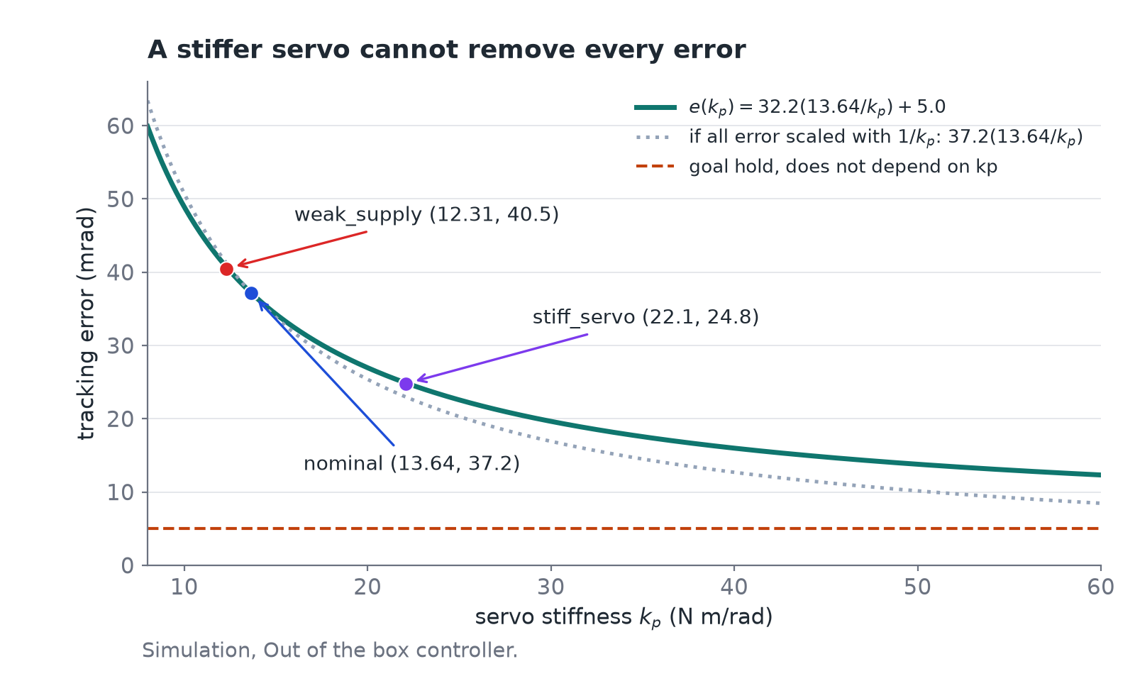
So even an infinitely stiff servo would still leave the goal hold, and on the real arm it would also leave the dead time. On top of that, a very stiff loop brings its own problems. The servo can't push more than about 5.1 N·m, so with a huge even a tiny gap asks for full torque and the motor ends up switching between pushing as hard as it can one way and the other. The encoder also only reads whole ticks, and every time the reading changes by one tick the torque jumps by times that tick, so the joint chatters between two ticks. And because the information the loop acts on is always a little old, a stiff loop pushes hard on a position that has already changed, overshoots, and then overshoots the other way. In practice, an outer gain of 4 stays stable and a gain of 100 oscillates.
Simulator against measured
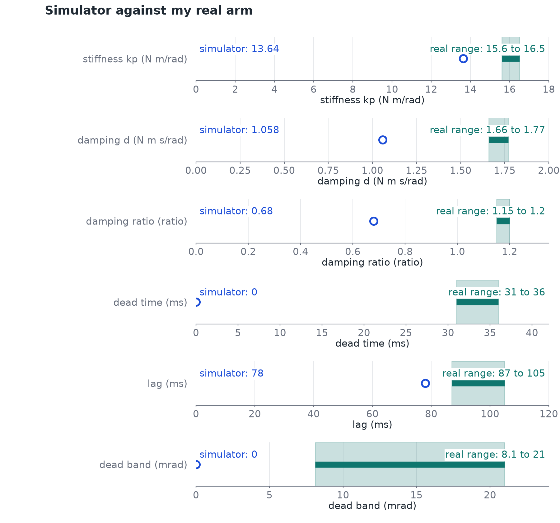
Most numbers in this article come from one of three places: the simulator, a data sheet, or my own arm, and they don't always agree. This table puts the main constants of the equation side by side.
| Constant | Simulator | Measured on my arm | Source |
|---|---|---|---|
| Stiffness (N·m/rad) | 13.64 | 15.6 to 16.5 | step test |
| Damping (N·m·s/rad) | 1.058 | 1.66 to 1.77 | step test |
| Damping ratio | 0.68 | 1.15 to 1.20 | step test |
| Dead time (ms) | about 0 | 31 to 36 (step), 15.6 to 26.6 (fit) | step test, servo fit |
| Lag (ms) | 78 | 87 to 105 | servo fit |
| Dead band (mrad) | none | 8.1 to 21.0 | servo fit |
| Torque clamp (N·m) | 5.107 | simulator |
The simulator values aren't measured on my arm. They come from a motor model of the 12 V STS3215 fitted by the open-source BAM project, with LeRobot's P = 16, and the 5.107 N·m torque limit comes from the same model. The measured column comes from a step test and a servo fit on my own arm.
The real servo is stiffer, more damped and later than the simulated one, which is a big part of why the controllers I tuned in simulation behaved differently on the arm.
What's next
So the arm misses because the servo needs a gap to make torque, every term of the equation needs a bit more of it, and the servo adds delays and limits of its own. Part 2 is about the sensor side: what the ticks do to a controller, and how to see the joint more finely than one tick. Part 3 writes one general formula for the goal, and shows that each controller I built is that formula with some terms switched off. Part 4 is about learning: where a neural network fits, and why it should learn only what the physics misses.