I own an SO-101 arm. I wanted to understand how a number sent from my laptop becomes a movement, and how joint angles determine where the gripper ends up. Why I'm learning robotics is a separate post.
How do we describe the arm?
Here is the Franka Panda used in my ManiSkill experiment. Its seven arm joints rotate; the fingers slide. The names below describe their motions, alongside the model's joint numbers.
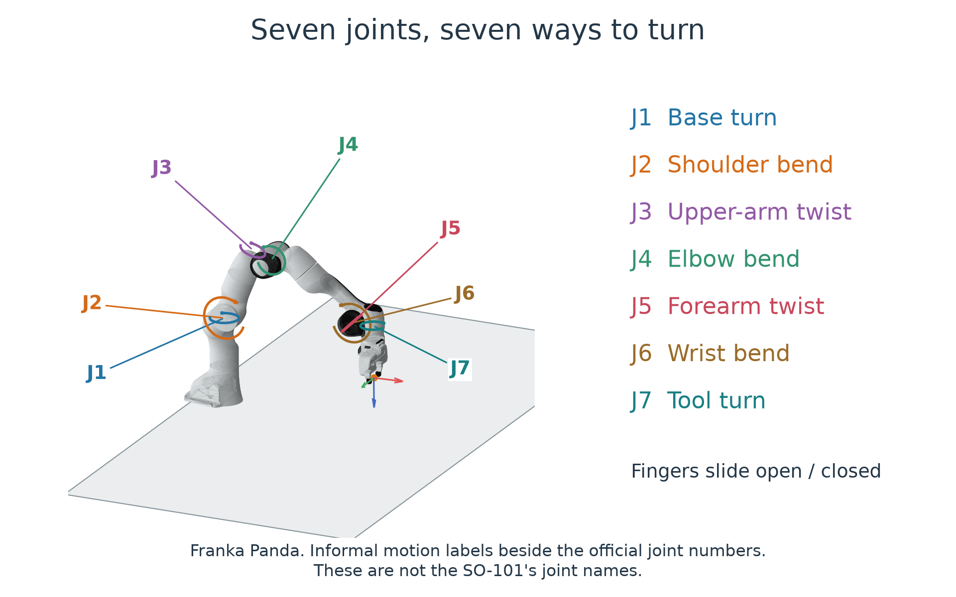
We could record the Cartesian position of every joint. But those coordinates are constrained by the rigid links, and joint-center positions alone miss rotation about a link's axis. A simpler description is the vector of joint angles, . Given the robot's geometry, these determine the positions and orientations of its arm links.
My SO-101 has five arm joints and a gripper actuator. An encoder inside each smart servo measures its angle. The arm's angles are its configuration. Its mechanical state also includes joint velocities, .
Watch the wrist rotate. The joints before it stay fixed; the gripper's pointing direction alone does not describe this motion.
Optional deep dive: how does the encoder find the angle?
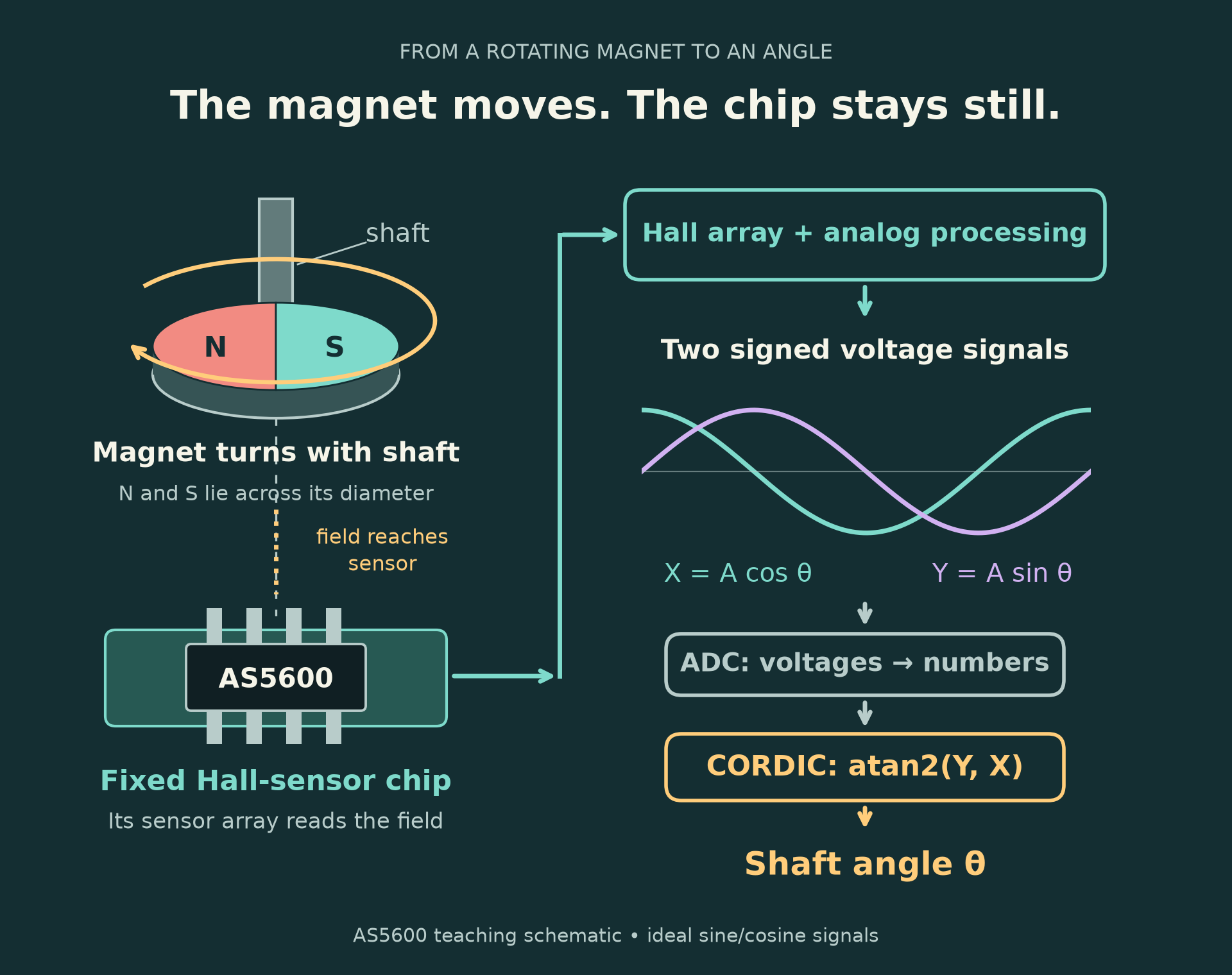
The magnetic encoder was one of the details I found most clever. A magnet turns with the shaft while a sensor chip stays fixed beneath it. Take the Hall-based AS5600 as an example.
A ready-to-connect Seeed Grove board with this chip was listed at US$6.50 for one on September 28, 2026, before tax and shipping. I find it remarkable that this much sensing and computation fits on a board that costs so little.
The Hall effect turns a magnetic field into a voltage. Current flows through a semiconductor; the field pushes the moving charges sideways, creating a voltage across it. As the magnet turns, the sensor array and its electronics produce two signed signals, a quarter-cycle apart:
Here is the signal amplitude and is the shaft angle. The two signals act like perpendicular coordinates. The rotating magnetic field supplies the sine and cosine signals. The chip's job is to recover the angle.
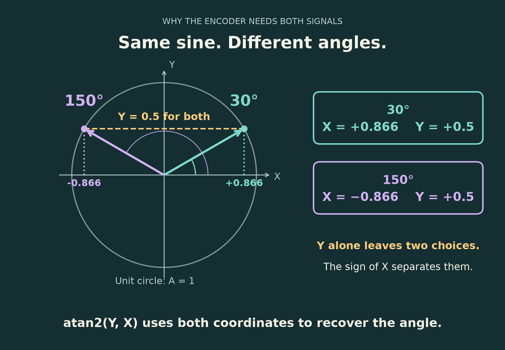
One signal leaves an ambiguity: 30° and 150° have the same sine. Their cosine signs differ, so the pair distinguishes them. The calculation is , which keeps both signs to identify the quadrant. TI's encoder guide explains this signal pair.
An analog-to-digital converter turns the voltages into numbers. How does a tiny chip recover the angle? Does it evaluate a Taylor expansion? That sounds like a lot of calculations.
CORDIC, short for Coordinate Rotation Digital Computer, does it with additions, subtractions, bit shifts, and a small lookup table. The AS5600 has a hardwired CORDIC block.
Imagine the measured vector is , pointing at roughly 30°. CORDIC rotates its coordinates toward the horizontal axis. Positive Y means turn clockwise; negative Y means turn back. It adds each signed turn to an angle estimate:
| Turn | Angle estimate |
|---|---|
| Clockwise by 45° | 45° |
| Back by 26.565° | 18.435° |
| Clockwise by 14.036° | 32.471° |
| Back by 7.125° | 25.346° |
Smaller corrections bring the estimate toward 30°. These are rotations of numbers in registers; the magnet supplies the original measurement.
Why do additions and shifts rotate a vector?
Start with . A 45° clockwise rotation gives . The update gives . Both point in the same direction. The second vector is simply longer.
Here is why. Write the original vector as . Turning clockwise by changes its angle to . The angle-subtraction identities give:
Factor out the same cosine from both coordinates:
For our turns between 0° and 45°, is positive. Multiplying both coordinates by this common factor changes the length while preserving the direction. We only need the angle, so we can leave that factor out.
Now choose . The remaining update becomes:
That is the whole trick. At , add and subtract the coordinates directly. At , use half of each coordinate. At , use a quarter. With scaled integers, these divisions become right shifts. For a counterclockwise turn, reverse the two signs. Both updates use the old coordinates.
This is an exact rotation followed by a stretch. The approximation comes from stopping after finitely many turns and rounding the stored numbers. Each chosen angle is computed ahead of time and kept in the lookup table. ST's CORDIC explanation.
Watch the same process with small integers. Start at , whose angle is about 29.995°. The first update gives and . We have turned too far, so the next step turns back. A right shift divides by a power of two and rounds down: 1399 >> 1 = 699.
The shift-and-add update
For the 30° example, start with , , and . At step , choose if , otherwise :
Both coordinate updates use the old values. At the first step, , this gives and . The negative Y tells us we overshot, so the next step turns back.
These updates scale the vector's length while preserving the direction of each rotation. For angle recovery, the direction is what matters. Once Y is close to zero, the accumulated angle is close to the original angle.
Is CORDIC actually faster than a Taylor expansion?
I implemented both and tested them on the same inputs. For Taylor, the series is:
Near , the powers shrink slowly. Range reduction means using an identity to replace the input with a smaller one, applying the series there, then restoring the known angle.
Here, first use signs and axis swaps to reduce the angle to between 0° and 45°, with between 0 and 1. If it is above 22.5°, compute its small offset from 45°. The tangent-subtraction identity gives:
So we can recover the angle with:
For example, becomes . We evaluate the series at about , then add 45°. Using the same three terms, :
- Directly at : about 39.81308°.
- At , then adding 45°: about 38.6598066°.
- Reference value: about 38.6598083°.
The same short polynomial becomes much more accurate because its input is smaller. Across the full reduced interval, the series now sees inputs with magnitude at most .
I set the error target to half a 12-bit encoder step: . All three methods passed on 1,114,197 coordinate pairs. These are native C++ results on an Apple M1 Max, using the median of 11 timing trials:
| Method | Steps or terms | Largest tested angle error | Time per angle in a batch |
|---|---|---|---|
| Basic Taylor | 326 terms | 0.04394° | 590.6 ns |
| CORDIC | 12 steps | 0.02798° | 10.78 ns |
| Taylor after extra range reduction | 3 terms | 0.01512° | 1.79 ns |
CORDIC was about 55 times faster than basic Taylor. But the range-reduced Taylor method was about 6 times faster than CORDIC on this laptop. I expected the shifts and additions to win; reducing the problem before doing the arithmetic mattered more here.
The appeal of CORDIC in a chip is its simple repeated step: shift, add or subtract, read a stored angle. A dedicated circuit can implement that directly. The AS5600 has such a CORDIC block.
Operation counts and benchmark setup
These counts describe the core calculation in the source code:
| Core calculation | Additions / subtractions | Multiplications | Right shifts | Table entries |
|---|---|---|---|---|
| CORDIC, 12 steps | 36 integer | 0 | 24 | 12 |
| Basic Taylor, 326 terms | 325 floating-point | 327 | 0 | 326 |
| Reduced Taylor, 3 terms | 2 floating-point | 4 | 0 | 3 |
CORDIC also makes 12 sign checks. Full-circle handling adds sign tests and possible negations. Returning its result as floating-point radians adds one conversion and one multiplication.
Both Taylor methods form a coordinate ratio with one division and handle signs and axis swaps. The reduced method sometimes uses a second division to replace with , then adds to the answer. The polynomial's input then has magnitude at most . Averaged over the timing inputs, this version uses 4 multiplications, 4.50 additions/subtractions, and 1.50 divisions, plus sign handling.
Operation types matter: a division and a shift have different costs. These are source-level counts; the compiler chooses the machine instructions. Loop bookkeeping and checksums are excluded from the counts.
Each method receives the same coordinate pairs, rounded to 30 fractional bits. Taylor receives exact floating-point versions of those values. Input preparation happens before timing. The reference is the system's double-precision atan2. Timing uses 65,536 fixed-seed inputs, 64 passes per trial, and rotating method order. Apple Clang 21 compiles with -O3 and floating-point contraction disabled. Media rendering was stopped during the timing run.
Implementations, raw timings, operation counts, and accuracy checks.
How does a motor follow an angle?
Sending “30°” does not tell a bare motor how long to turn. A servo, short for servomechanism, is an actuator with feedback: it compares a measured quantity with a target and corrects the error. In the SO-101, the smart servo packages the motor, encoder, driver, gears, and controller together.
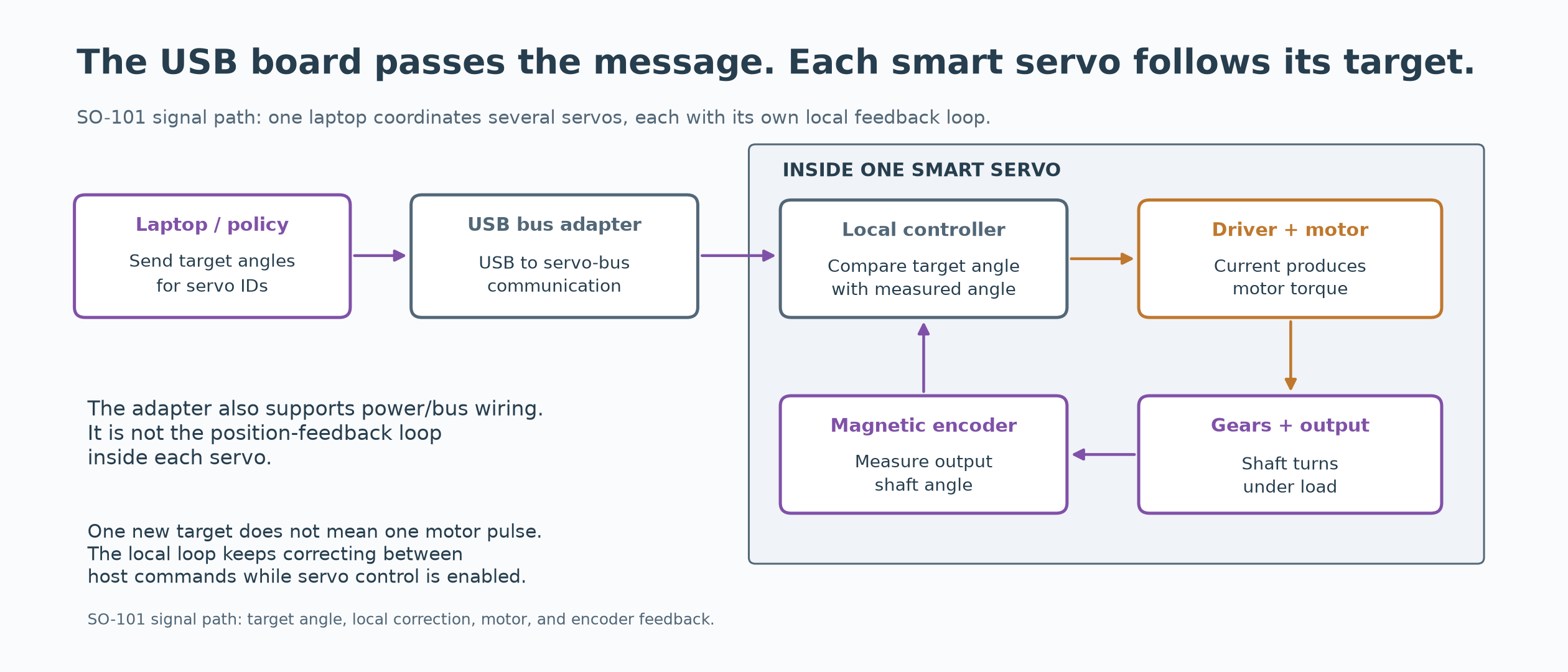
The USB board passes messages to the servo bus. Each servo runs its own feedback loop between laptop commands. A magnetic encoder senses a rotating magnet to measure angle. The adapter documentation and STS3215 datasheet describe this hardware.
Suppose the desired angle is and the measured angle is . The error is . The target command is an action; the encoder reading is an observation of the current state. A standard PID controller turns that error into a drive command:
Here is the requested motor drive. The three gains set the strength of three corrections:
- Proportional: react to the current error. A larger gap produces a larger correction.
- Integral: accumulate error over time. The stored correction keeps producing torque even after the error reaches zero.
- Derivative: react to changing error. For a fixed target, , so this term opposes motion and helps brake before overshoot.
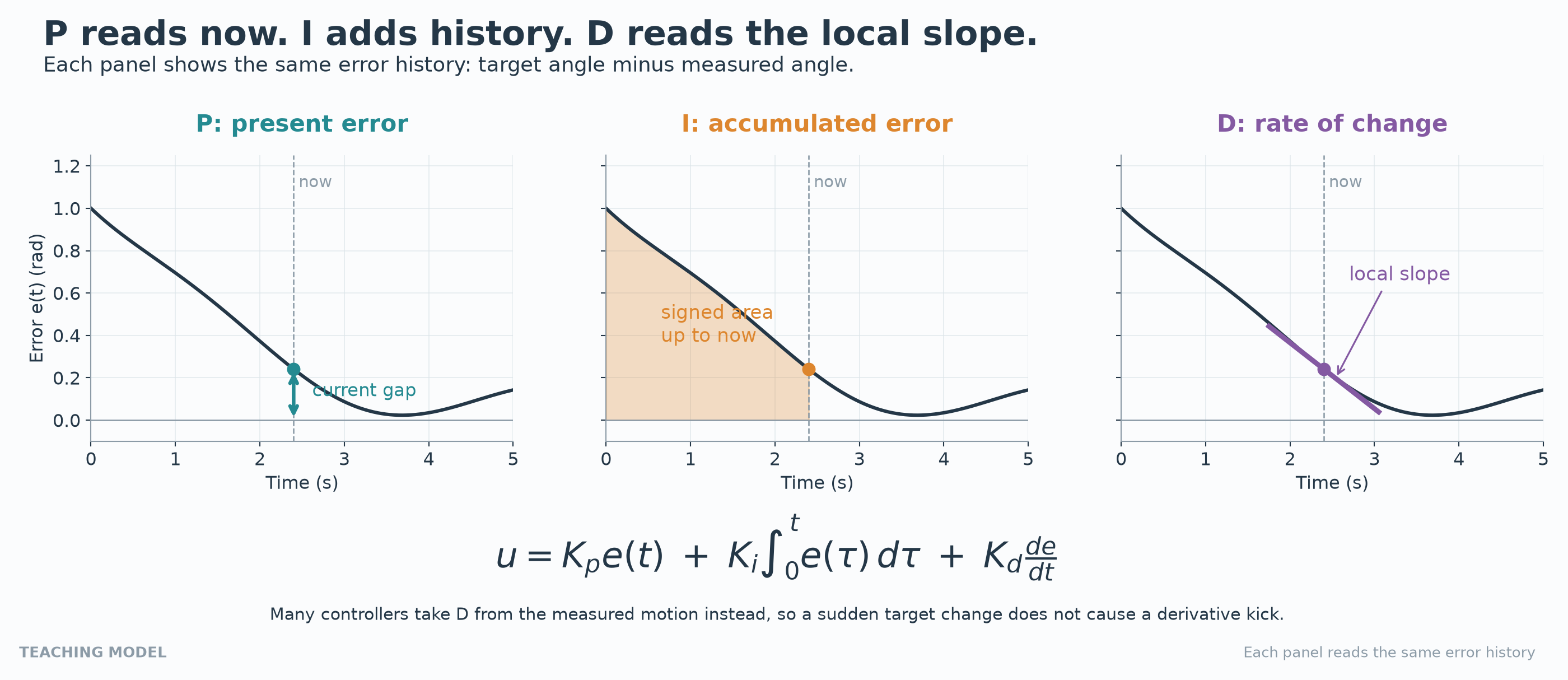
Why keep past error? Imagine the arm stops a little below its target under a steady load. The proportional correction balances the load, so the arm stays still. But the error is still positive. The integral keeps growing, adds more torque, and lifts the arm closer to the target. Once the error reaches zero, the integral stops growing. Its stored value supplies the torque that holds the load.
What happens if we remove P, I, or D?
I simulated one rotary link under a constant clockwise load. Every run starts at rest at 0°, with a target of 45.8°. I kept the same gains and set one to zero. This is an ablation test: change one part and watch what happens.
| Controller | What happened | What the missing term was doing |
|---|---|---|
| Full PID | Reaches within 2% of the target in 2.20 s and stays there | All three corrections work together |
| Remove I | Stops 7.16° short | I supplies the holding torque at zero error |
| Remove D | Overshoots by 64.3% and rings; settles in about 30 s | D brakes the motion |
| Remove P | Initially falls away from the target, then oscillates more and more | P supplies an immediate correction toward the target |
The no-I result has a simple explanation. At rest, D is zero, so P must balance the 2 N·m load. With , this requires an error of rad, or 7.16°. With I enabled, the stored integral supplies that torque while the error approaches zero.
Removing D still leaves passive friction, so those oscillations eventually decay. Removing P produces growing oscillations with these gains. The arm and load stay fixed; each run removes one gain and keeps the others unchanged.
Simulation setup and checks
The link rotates in a horizontal plane with inertia kg·m² and viscous friction N·m·s/rad. A constant external torque of 2 N·m opposes positive rotation. The controller supplies torque directly:
The initial angle, velocity, and integrated error are zero. Each ablation sets one gain to zero. Actuation is continuous, with unlimited torque. The derivative uses measured velocity to avoid a kick when the target changes.
I integrated at 2 ms, repeated at 1 ms, and checked against the exact solution of this linear system. Angle differences were below rad. Settling means staying within 2% of the target over an 80-second run. The system's poles confirm that the no-P response is unstable.
Why does the arm overshoot?
The clips use the same target and clock. An underdamped joint overshoots and oscillates. An overdamped joint approaches slowly without oscillation. Critical damping is the boundary between those two responses in this ideal second-order model.
The equation behind the animation
For a single joint with inertia , viscous friction , and PD control at a fixed target:
measures resistance to angular acceleration. measures friction proportional to speed. The dimensionless damping ratio (zeta) compares damping with its critical value: between 0 and 1 is underdamped, 1 is critical, and above 1 is overdamped. The animation assumes positive inertia and proportional gain and omits integral action, gravity, delay, and contact.
Changing the load or arm configuration changes the response even with the same controller gains. Gains can differ by joint or vary with pose and load. PD control and damping.
Joint angles or a gripper target?
The servo accepts a joint target. But I usually care about the gripper: “put it at this point above the cup.” These are two descriptions of the task.
Joint space contains configurations . Task space contains the quantity we want to control: here, the gripper position . Later we'll add orientation.
Forward kinematics is a function , with . For this arm, it is non-injective: distinct configurations can put the gripper at the same point. It is not surjective onto because reach is bounded. It is surjective onto its image. With joint and collision constraints, the reachable position workspace is .
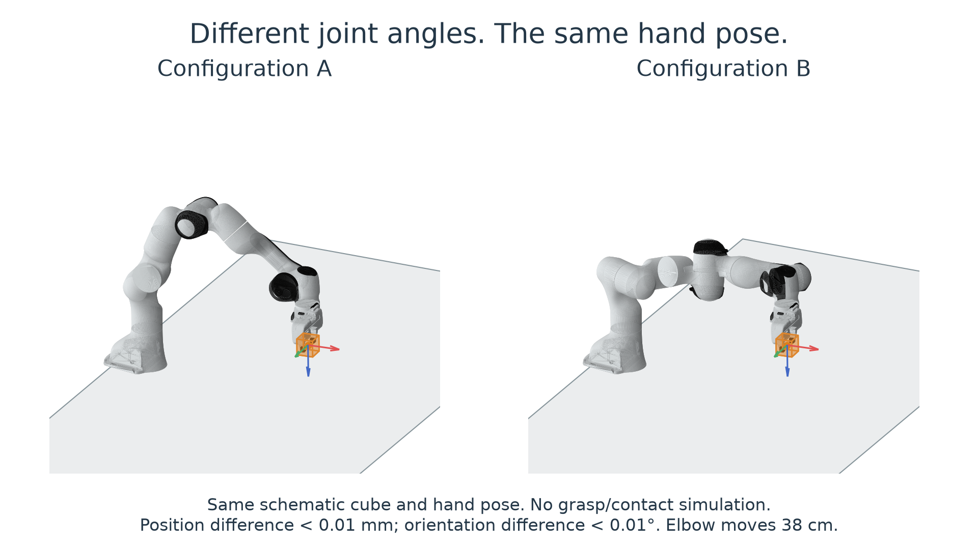
The gripper has the same position and orientation in both configurations, while the elbow moves about 38 cm. The cube marks the shared target.
Inverse kinematics (IK) searches for joint angles matching a target:
imposes joint limits and the chosen collision constraints. The answer may be empty or contain many configurations. IK is not a single-valued inverse function, and an IK solution is not a motion path.
This ambiguity matters during motion. A numerical solver seeded with the current configuration tends to select nearby solutions. Otherwise, repeated solves can choose different branches and produce abrupt target jumps.
On the left, the animation alternates between two valid solutions. On the right, it selects the solution nearest the previous one.
How do we describe gripper position mathematically?
Seven joints make the geometry look complicated. Let's start with a simpler arm: a fixed base and links that all bend in one plane.
Start with one link of length at angle . Its endpoint is . Then add a second link, then a third:
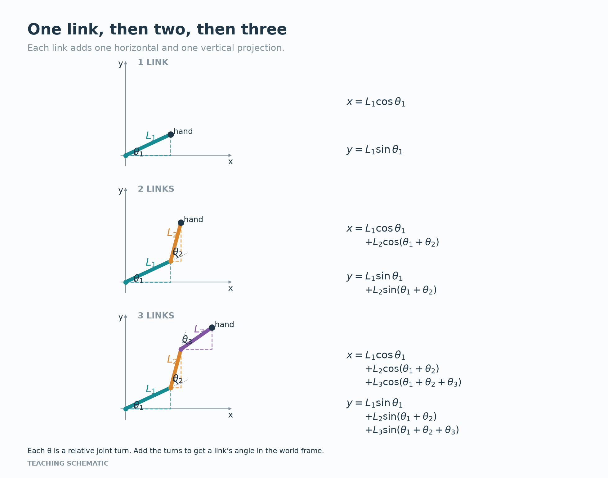
The second link's absolute angle is . The third's is . The diagram uses planar coordinates . For the vertical arm plane, rename them . For links:
Here is shoulder height and is the signed horizontal reach. This gives a convenient parametrization of the simplified SO-101 geometry. From the side we compute ; from above, shoulder pan rotates that reach into :
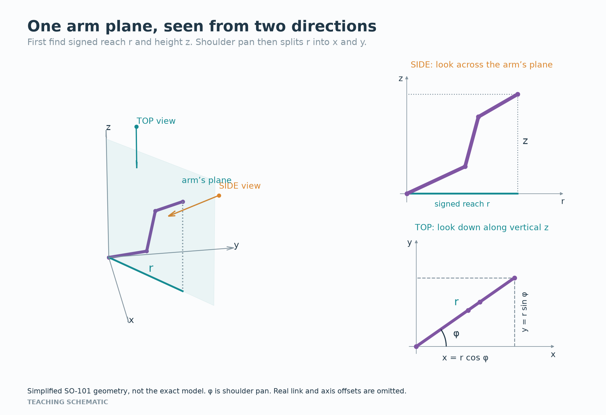
Folding past the pan axis can make negative; horizontal distance is .
Try two links with lengths 1 and 0.8. The shoulder angle is . The elbow adds , so the second link points at . In the top view below:
Two joints. One position.
Turn the joints. Watch the tip move.
Link lengths: 1 and 0.8 units. Angles in degrees.
How does a small joint turn move the gripper?
Once is defined, differentiate it:
That derivative is the Jacobian. For position control:
For example, is the change in gripper X per small change in joint 2, with other angles fixed. Repeat for every coordinate and joint. Column 2 gives the resulting 3D velocity per unit joint velocity.
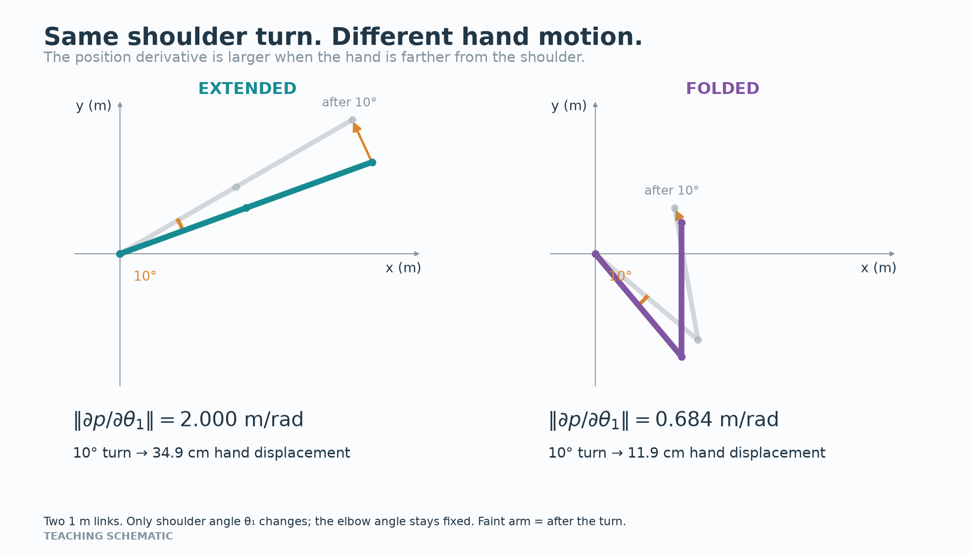
The Jacobian is a matrix-valued field over configuration space. Its value changes with the whole arm configuration. For small changes, .
At an interior point of , its image contains the attainable instantaneous position velocities. Its kernel contains joint velocities that preserve hand position to first order. Rank 3 means the position derivative is surjective.
I kept mixing up three words. Their roots helped me separate them:
- Kinematics comes from Greek kīnēma, “motion,” from kīnein, “to move.” It describes positions, velocities, and accelerations without considering the forces that produce them. Word origin.
- Dynamics comes from Greek dynamis, “power.” It connects forces and torques to motion. The same arm configuration with different velocities is a different state: a moving arm may need braking where a stationary arm does not. Word origin.
- Proprioception combines Latin proprius, “one's own,” with the ending of reception, “receiving.” It means sensing your own body's state. For a robot, joint encoders provide this kind of information. Word origin.
Where can the hand actually go?
Looking at my arm on its table, I wondered about the whole reachable region. It cannot pass through the tabletop or its own links. The thickness of the hardware matters, as do objects around it.
My first guess was part of a sphere. Suppose pan is limited to 180° and the arm stays above a table. That leaves half of the upper hemisphere: a quarter-ball envelope.
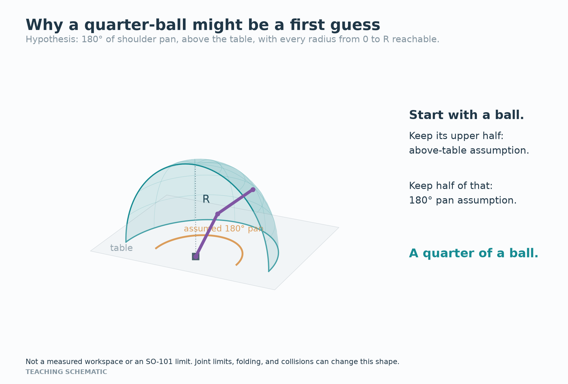
Even two ideal links cannot fold closer than to the shoulder. Joint limits, thickness, and obstacles can exclude more space.
I tested the question on the Franka model. For each sampled set of joint angles, I computed the gripper position and checked collisions. This samples the workspace .
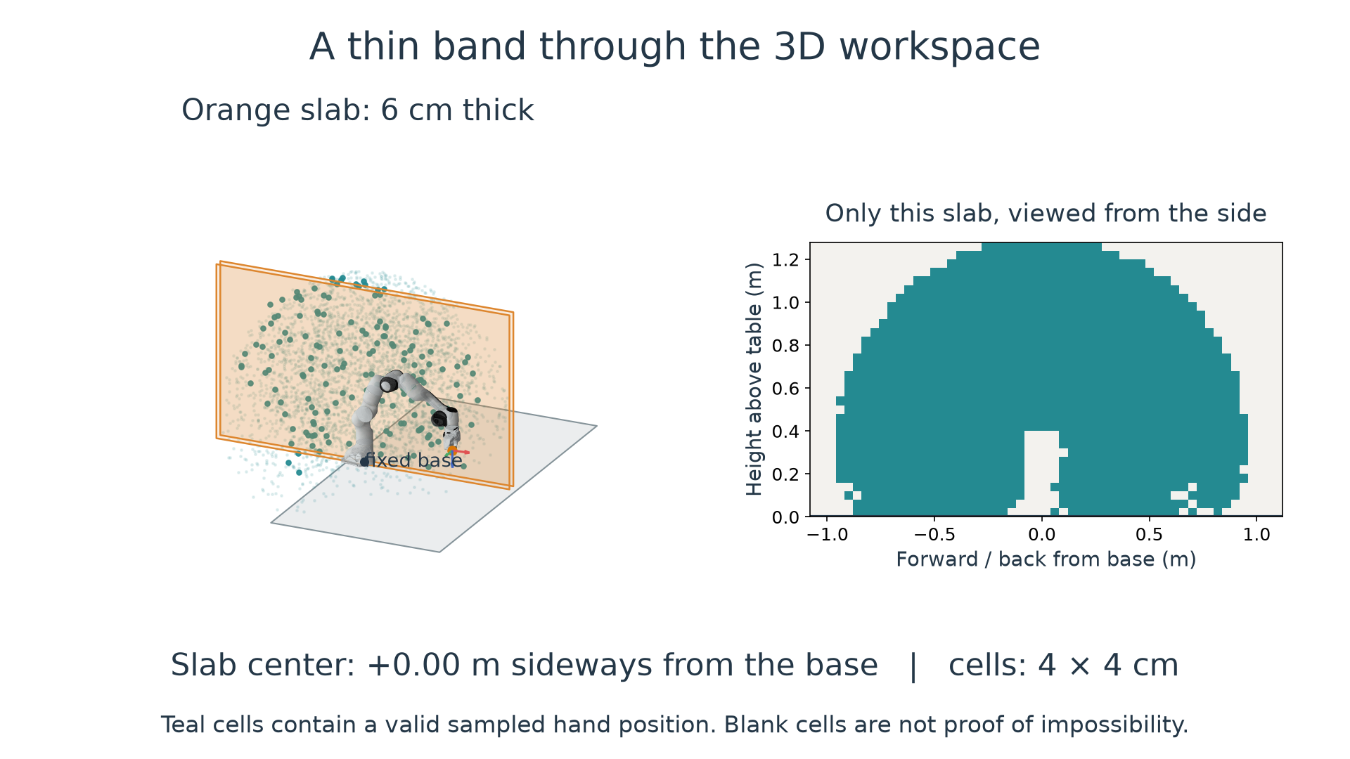
The orange slab is a 6 cm thick band, moving sideways through the cloud. The right panel looks straight at that band: signed forward/back position relative to the base versus height, grouped into 4 cm cells. It shows only the above-table portion of the data. Teal means at least one valid hand position was found in that cell. Blank cells contain no accepted sample. The arm stays fixed as a spatial reference while the slab scans the cloud.
What did the experiment actually measure?
I sampled 300,000 configurations uniformly within the seven arm joints' model limits, with the fingers open. Of these, 263,270 passed the recorded self-collision and environment checks. The table, ground, and task cube were included. Uniform joint sampling is not uniform sampling of hand positions.
Sampling gives a partial picture of the workspace; blank regions may still contain reachable points. Model, joint limits, collision rules, data, and reproduction.
Reaching the stem is not enough
Suppose I want to grasp a wine glass by its stem. Reaching the stem's position is only part of the problem: the gripper must approach in a useful orientation, with room for its fingers.
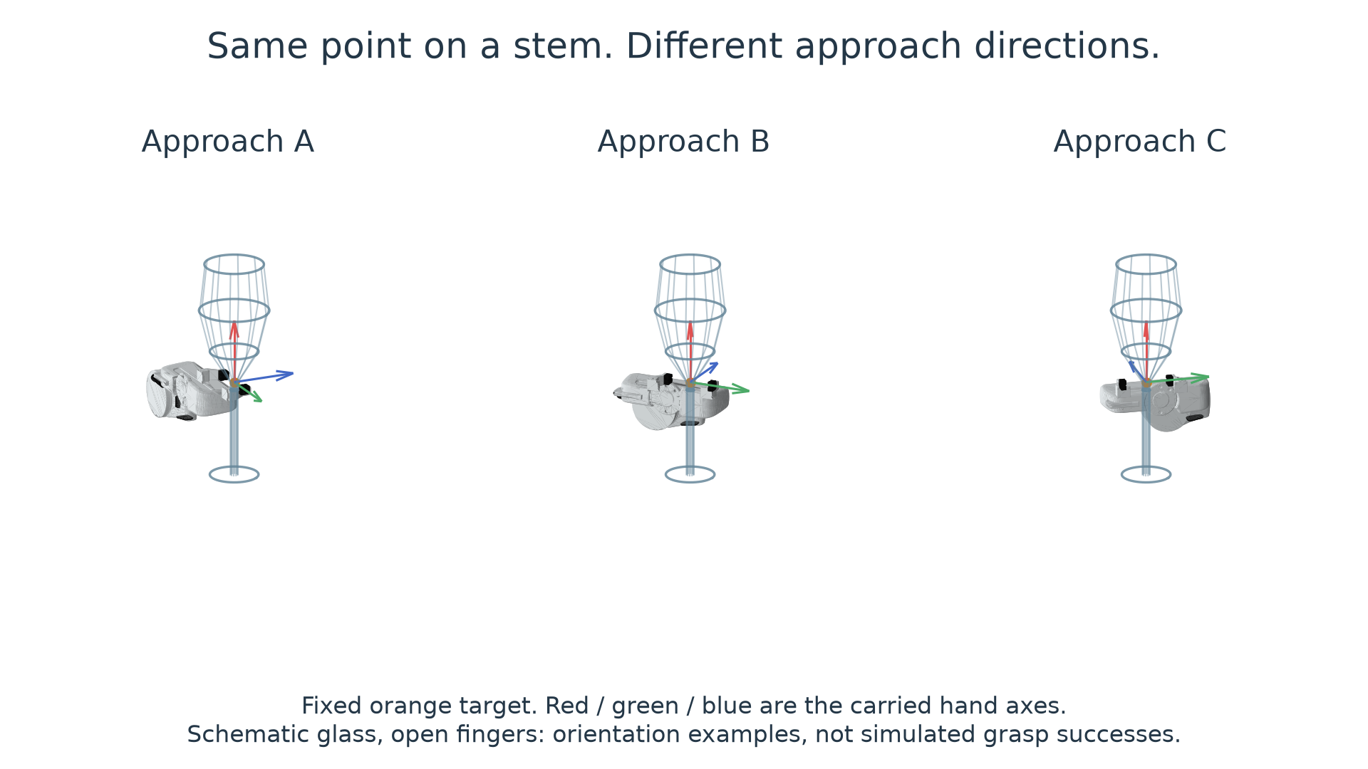
In the simulation, the hand keeps the same target point while changing orientation.
So the hand needs more than an XYZ point. Attach an orthonormal frame to it. Express its three unit axes in world coordinates and put them in the columns of a matrix:
This is a rotation matrix, . Position and orientation together give a pose, . means aligned axes.
Imagine looking straight down at the arm in the video. Put two perpendicular arrows on the gripper, lying in the tabletop plane: X points right and Y points up the page. Now turn both arrows counterclockwise by . Where does each arrow point? Those coordinates become the columns of the rotation matrix.
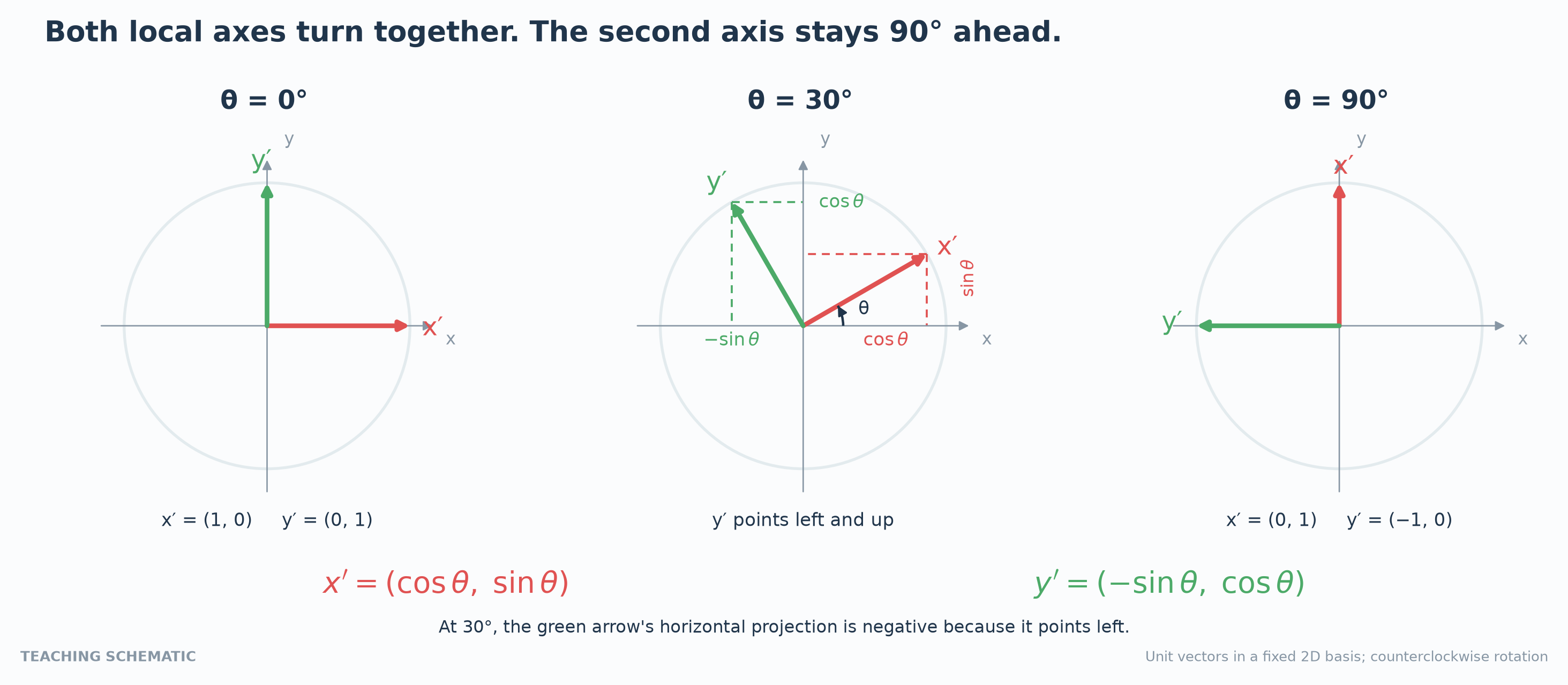
The first axis becomes . The second stays ahead, hence . At 90°, it points left. A twist about the gripper's local Z axis composes as .
The pose workspace contains reachable position-orientation pairs. The dexterous workspace contains positions reachable at every orientation.
Who chooses the next target?
We can now work backward from the motor. In the SO-101 position-control setup, the servo needs a joint-angle target. It cannot interpret “grasp the cup.” Something above it must turn that goal into commands.
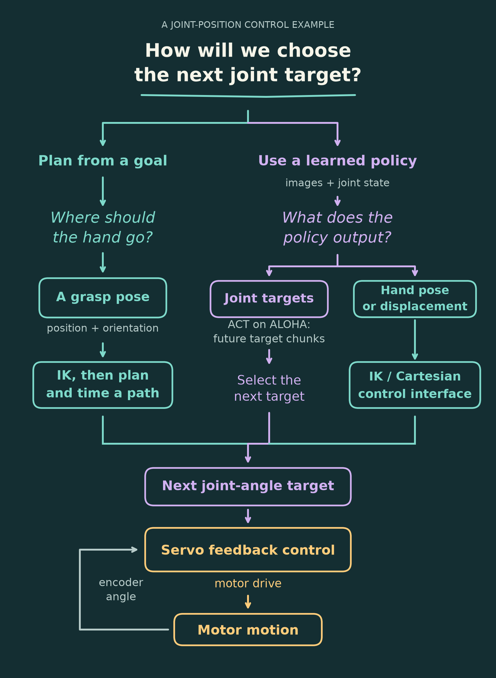
Classical planning: choose a grasp pose, use IK to find a joint configuration, then plan and time a collision-free path into intermediate joint targets. IK chooses an endpoint; planning supplies the motion between endpoints.
ACT: predicts a chunk of future joint targets from images and measured joint positions in the original ALOHA setup. Execution selects or combines chunk targets as fresh observations produce new predictions. Temporal ensembling can combine overlapping chunks. ACT paper.
Learned task-space targets: a model can instead propose a hand pose or displacement. An interface then uses IK or a Cartesian controller to produce commands the robot accepts.
One way to combine models is to let a vision-language model (VLM) select a high-level goal and a vision-language-action model (VLA) predict motion commands. Some VLAs take images and instructions directly; their outputs may be joint or task-space commands. PaLM-E, OpenVLA.
Other robots accept velocity or torque commands. The common requirement is to match the controller's interface, units, frame, and timing.
Sources and inspiration. Jacob Rothschild's control article helped inspire this report. Also: Modern Robotics, SO-101 joint guide, and asset credits and licenses. Robot renderings use the simulated model; the planar and control animations are teaching schematics.